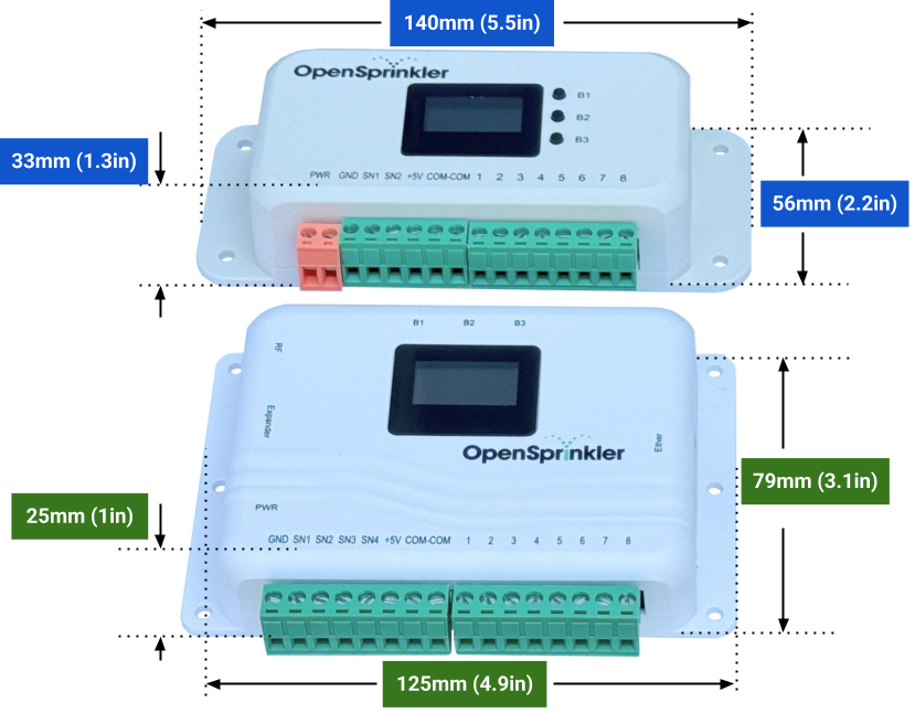
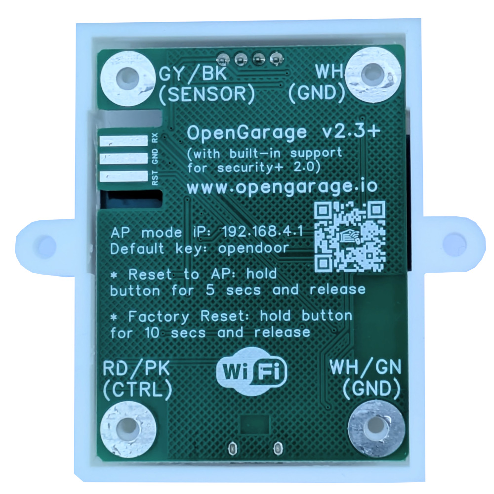
Exciting news! We’re preparing to release a new hardware revision of OpenGarage: version 2.3+. This will be the first OpenGarage to include native support for Security+ 2.0, eliminating the need for an external Security+ adapter. The hardware form factor is identical to OpenGarage v2.2, but with enhanced circuitry and software library courtesy of the open-source work of Ratgdo.
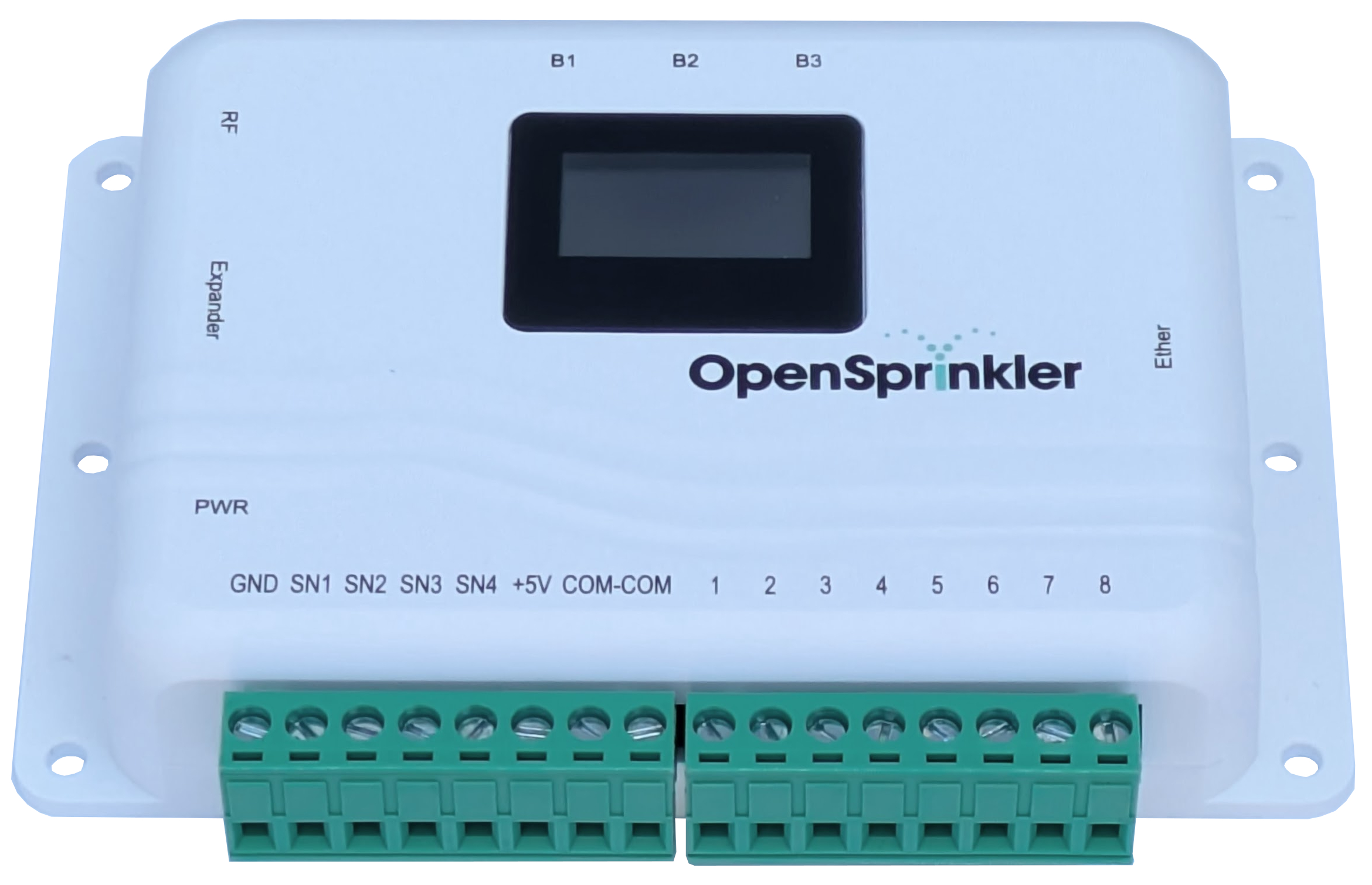
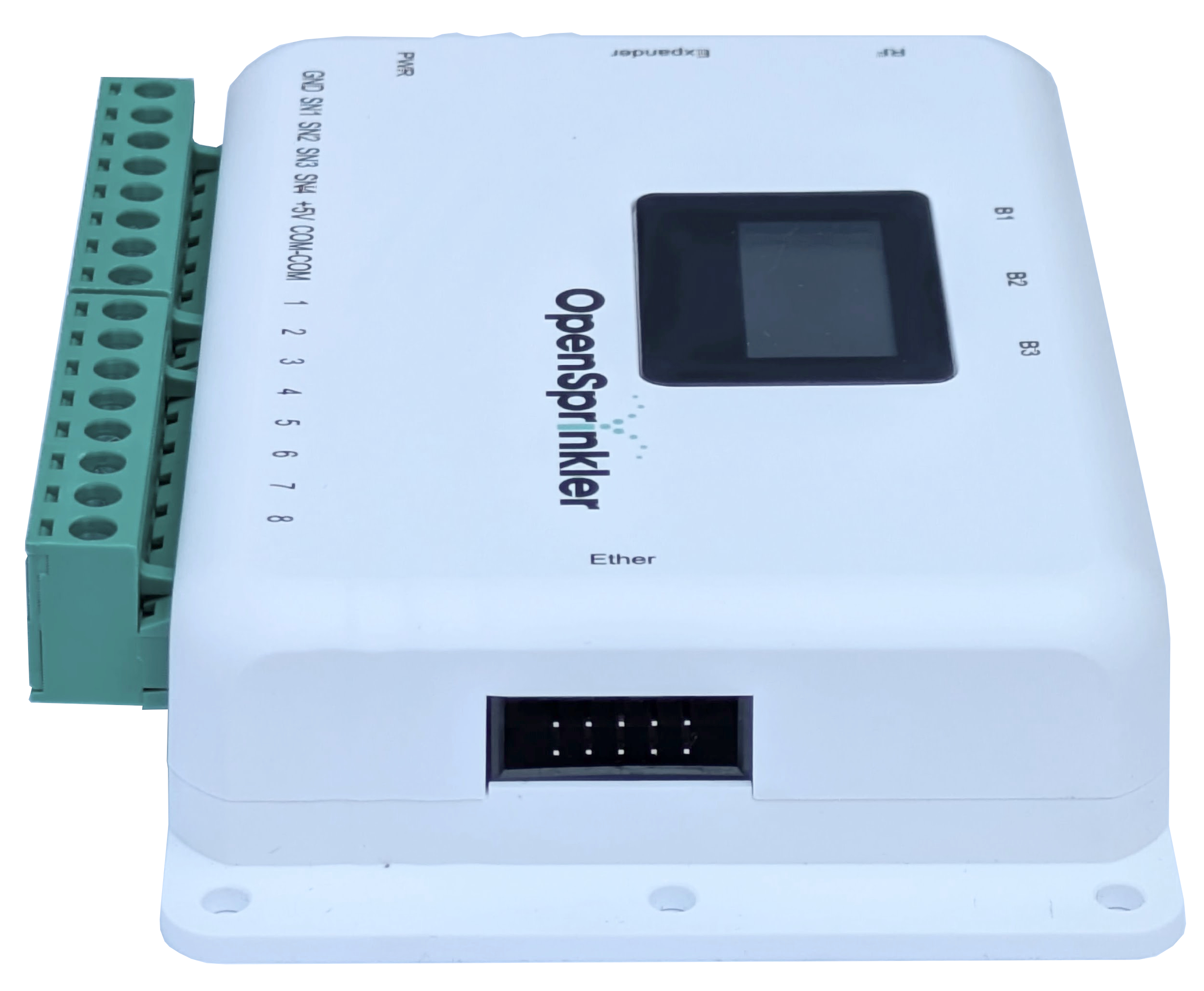
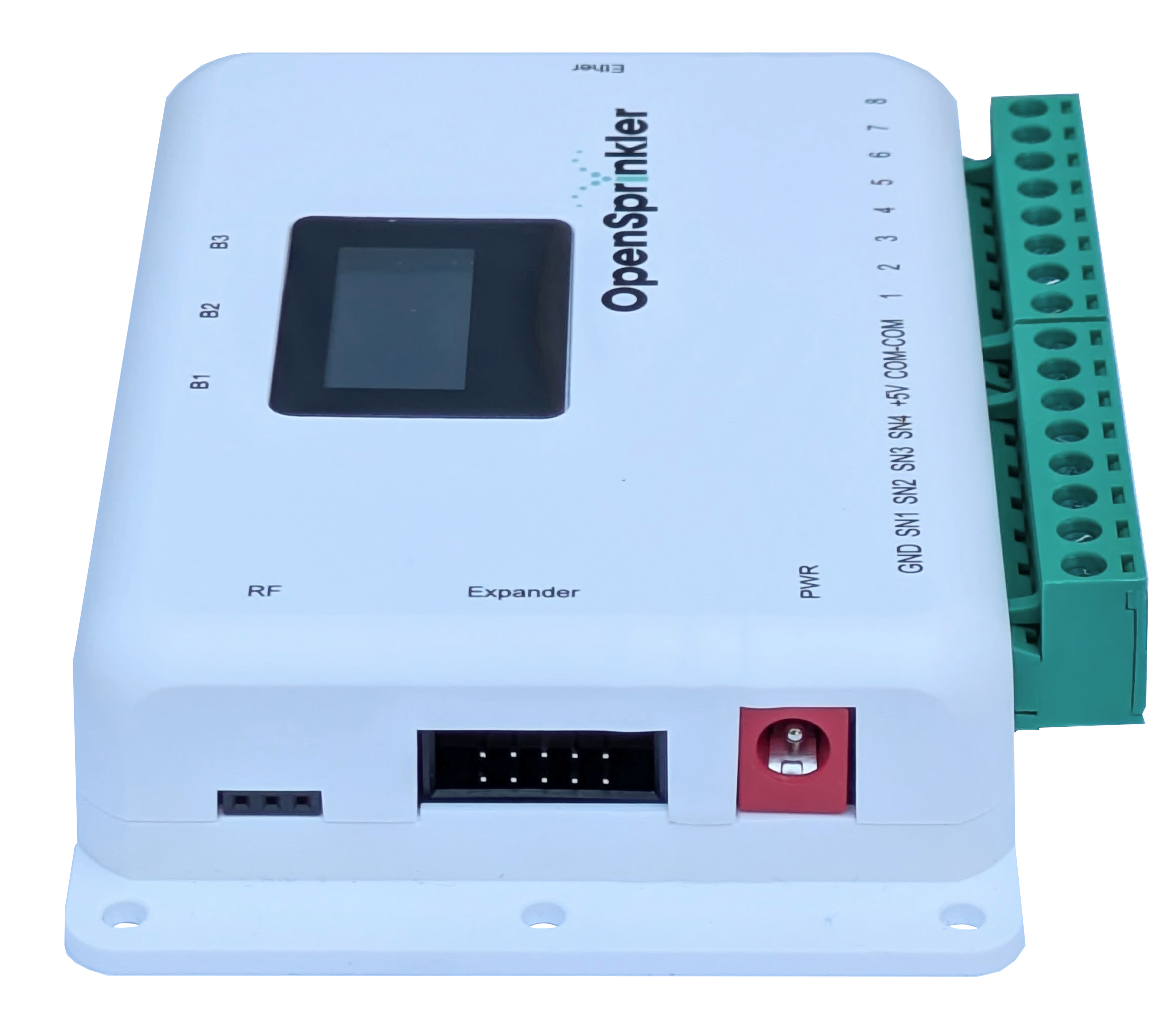
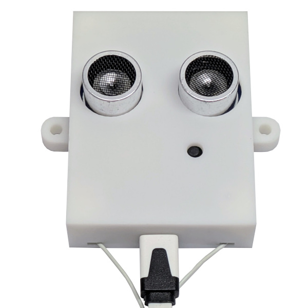
With this upgrade, OpenGarage can communicate directly with Security+ 2.0 garage door systems, enabling new capabilities such as reporting partially open status and controlling the opener’s light. Here’s a sneak-peek photo of version 2.3+:
FAQ
Q: What is Security+ 2.0?
A: Security+ 2.0 is a garage door opener technology introduced by Chamberlain around 2011 and sold under the LiftMaster, Chamberlain, and Craftsman brands. It uses rolling-code encryption for both remotes and wall button controls, providing stronger security and more reliable signals.
You can usually identify a Security+ 2.0 opener by its yellow “learn” button (and often a yellow antenna too). If you’ve purchased a garage door opener of the above brands in the last several years, there’s a good chance it uses Security+ 2.0. If you are not sure, take a look at your opener’s user manual, usually it will explicitly mention the term Security+ 2.0.
Unlike older systems, which worked by simply shorting the two button wires, Security+ 2.0 enforces the use of encoded signals. This allows not only open/close commands, but also richer feedback such as whether the door is partially open or the light is on.
Q: Why couldn’t earlier versions of OpenGarage support it directly?
A: Previous versions (like v2.2) relied on shorting the two button wires — which no longer works with Security+ 2.0. To control those systems, you had to use an external adapter (e.g., the Security+ 2.0 adapter that we sell) as a “middleman.” When the two wires on the adapter are shorted, it generates encoded signals accepted by the opener.
Q: What is Ratgdo?
A: Ratgdo (Rage Against The Garage Door Opener) is an open-source project developed by Paul Wieland. It allows a microcontroller (such as an ESP8266) to directly speak the Security+ 2.0/1.0 protocols via GPIO pins. In effect, Ratgdo replicates what a proprietary Security+ 2.0 adapter does — enabling direct open/close/stop commands, door status reporting, and even light control.
Q: What hardware changes are in OpenGarage v2.3+?
A: v2.3+ incorporates the same type of control circuits shared by the ratgdo community (see rat-ratgdo). It uses two MOSFETs — one for transmitting, one for receiving — to safely interface with the opener’s signal/button wire (typically 12 V DC).
⚠️ Important: Because of this design, v2.3+ is NOT compatible with legacy openers that use AC (e.g., 24 VAC) on the control /button wires. Using it on those systems could damage the circuitry. For those setups, OpenGarage v2.2 remains the recommended model.
Q: When will OpenGarage v2.3+ be available?
A: We’re now accepting pre-orders, with shipments expected no later than early October 2025.
Q: Does v2.3+ still use the built-in ultrasonic distance sensor?
A: Since Security+ 2.0 directly reports the door’s open/close status, there’s no need to rely on the ultrasonic sensor for that purpose. In Security+ 2.0 mode, v2.3+ will not use the sensor for door status, but it will continue using it to detect vehicle presence in the garage.
Q: Will OpenGarage v2.2 still be sold?
A: Yes. Since v2.2 is compatible with legacy openers, including both AC and DC systems (via its onboard solid-state relay), we’ll continue offering it alongside v2.3+.
Q: If v2.2 works with an external Security+ 2.0 adapter, why upgrade to v2.3+?
A: Two key reasons:
- More features — v2.3+ enables additional features such as reporting partial open status and toggle the opener’s light, which Security+ 2.0 adapters can’t provide.
- Lower cost — buying v2.2 plus an external adapter costs more than a single v2.3+.
Bottom line: Choose v2.3+ if your garage door system is made by Chamberlain, LiftMaster, or Craftsman. For all other brands, use v2.2. (Technically, any system with button wires that output DC below 20 V can use v2.3+, but it offers no benefit on other brands since they don’t support the Security+ protocol.)
Q: Can I modify my existing v2.2 to support Security+ 2.0?
A: In theory, yes — by adding MOSFETs and resistors. But unless you’re experienced with soldering, we don’t recommend it.
Q: What about Security+ 1.0?
A: Security+ 1.0 (mid-1990s–2010) was Chamberlain/LiftMaster’s first rolling-code system. It used colored learn buttons (purple, red, orange, green), but shorting the two wires still worked. Its status reporting is limited compared to 2.0. Ratgdo also supports Security+ 1.0, so with v2.3+ you can still read door status and control the opener’s light on those systems.
Q: I just bought an OpenGarage — can I exchange it for v2.3+?
A: Yes. Purchases made within the last 30 days qualify for our no-questions-asked return/refund policy (see our terms and conditions).
Summary
✨ With v2.3+, OpenGarage now natively supports the Security+ 2.0 technology — no additional adapters required, more features unlocked, and the same compact design!