Feed on
Posts
Comments

Introduction

In the world of irrigation, 24 VAC sprinkler solenoids have been the industry standard for decades, and the traditional way to power them is equally old-school: a bulky 24 VAC wall transformer. It works, but these transformers are heavy, expensive, and inefficient. Their output voltage is unregulated, and their overload and short-circuit protection is primitive. They are also tied to the mains standard—a transformer designed for 120 V mains cannot be directly used on a 230 V outlet in another country.

Contrast that with modern DC switch-mode power supplies. They are lightweight, cheap, efficient, and protected against common faults. Better still, they accept 100-240 V input, so work anywhere in the world.

Among DC power sources, one has become nearly universal: USB-C. With Power Delivery (PD), a USB-C adapter is no longer just a 5 V phone charger. Instead, it can supply multiple voltage levels and ample juice for much heavier loads. Those that support PPS (Programmable Power Supply) further allow the voltage to be adjusted in fine increments. That raises an interesting question: can we ditch the traditional AC transformer and drive sprinkler solenoids from USB-C instead?

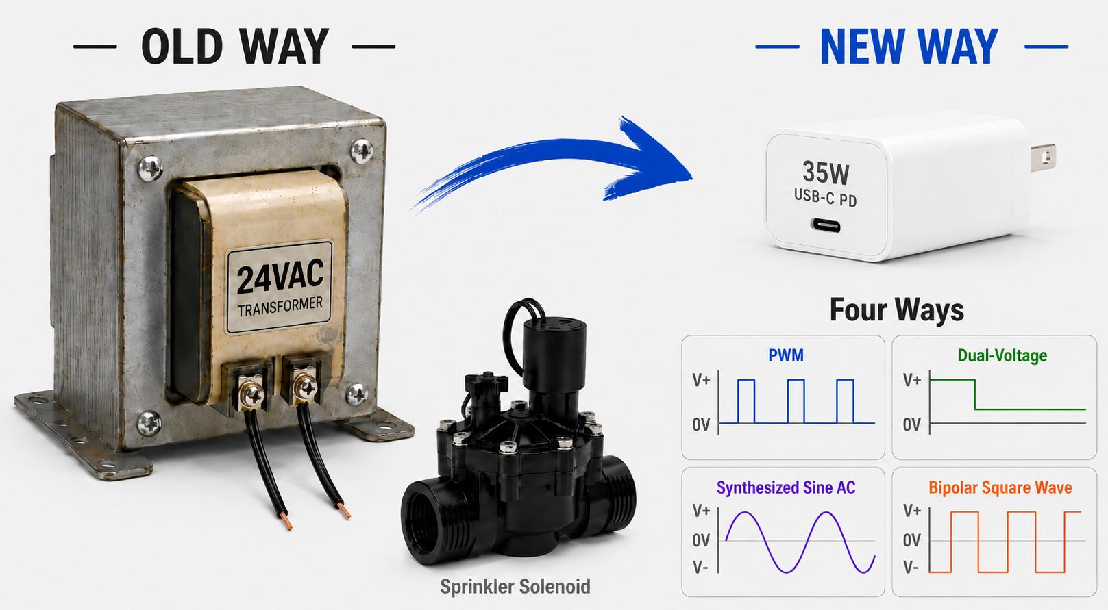
Yes—and there is more than one way! In this article, I will dive into four of them, summarized below:

Drive MethodDescriptionFrequencyDrive Waveform
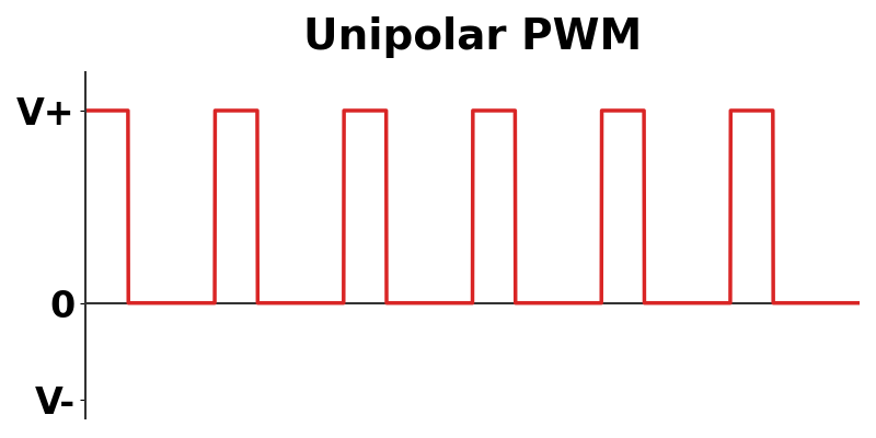
PWMControl effective holding current by PWM duty cycle1 kHz or aboveVoltage waveform for PWM
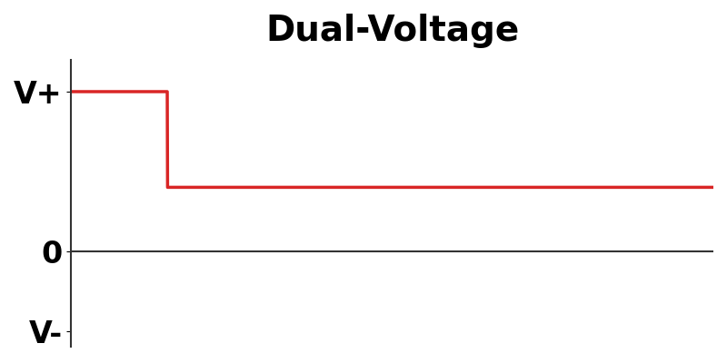
Dual-VoltageApply high voltage initially for pull-in, then drop to a lower voltage for holding.DC (0 Hz)Voltage waveform for dual-voltage
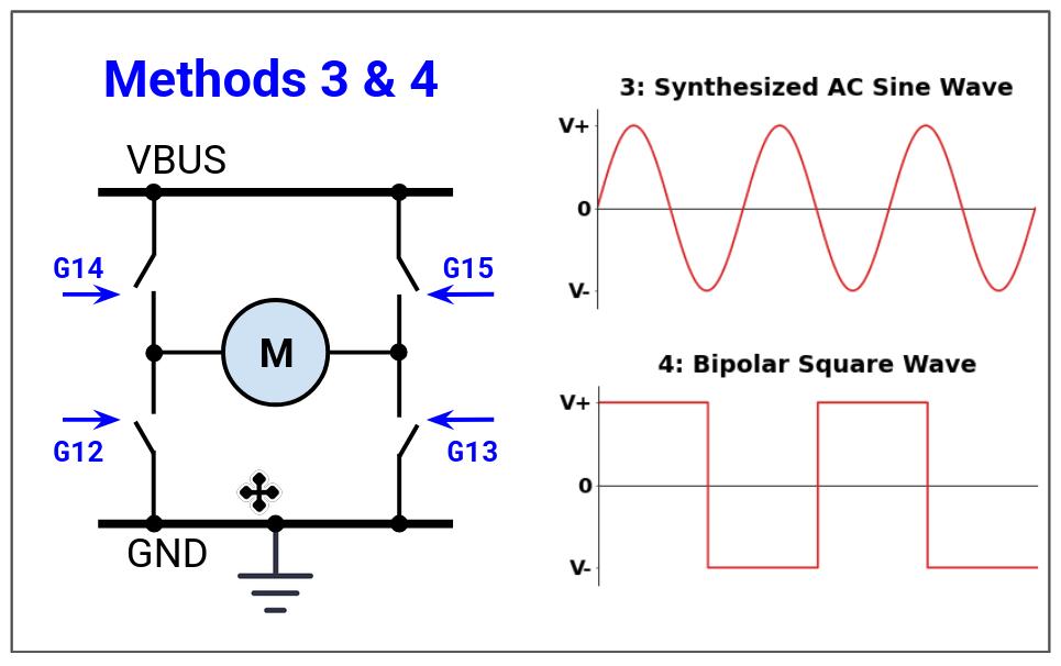
Synthesized Sine WaveUse an H-bridge to synthesize AC sine wave from DCCarrier: 40 kHz
Output: 60 Hz
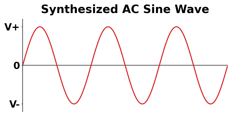
Voltage waveform for synthesized sine wave
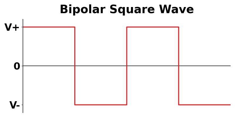
Bipolar Square WaveUse an H-bridge and alternate DC polarity to produce a square-wave 45 HzVoltage waveform for bipolar square wave

I built a small custom circuit to test all four, so rather than just talking theory, we can watch actual waveforms on the oscilloscope and take measurements at the solenoid.


The Electric Quirks of 24 VAC Solenoids

To begin, it helps to understand how sprinkler solenoids work electrically. I wrote a detailed article about this more than a decade ago in Understanding 24 VAC Sprinkler Valves. Below I summarize the important points.

A typical solenoid consists of a coil surrounding a spring-loaded iron plunger. Applying 24 VAC energizes the coil and pulls the plunger inward, which in turn opens the valve. Electrically, the coil can be modeled as a resistor in series with an inductor. Typical solenoid specs are:

  • Coil Resistance: 25–60 Ω
  • Inrush Current: 300–500 mA
  • Holding Current: 150–250 mA

Initially, the solenoid needs a fairly large inrush current to pull the plunger into the coil. Once seated, it can stay there with a smaller holding current. Under AC, this transition happens naturally because the inductance—and hence the inductive reactance and total impedance— increases significantly as the plunger pulls in. This also explains why a stuck or missing plunger leaves the inrush current flowing indefinitely, which can burn out the coil.

This behavior is one reason that simply replacing 24 VAC with a fixed DC voltage is not ideal. Under steady-state DC, the current is determined entirely by the coil resistance, and inductance no longer limits it. Therefore, a voltage high enough for reliable pull-in will produce unnecessarily high holding current. Conversely, a lower voltage suited for holding may not pull the plunger in at all.

Note: this article is specifically about conventional 24 VAC sprinkler solenoids, which are used in the vast majority of irrigation systems. Valves that run natively on DC do exist, including latching solenoids and motorized ball valves, but they are less common and more expensive than 24 VAC valves. For that reason, DC-operated valves are not the focus of this article.


The Four Methods

1. Unipolar PWM

Idea: Apply a fixed supply voltage high enough to pull the plunger in, and rapidly switch that voltage on and off. This reduces the average current through the coil to match the target holding current.

Reference: This is the approach Vinne used to convert his sprinkler system to DC, driving each solenoid with a DRV103 solenoid driver.

Design Parameters:

  • Supply Voltage. Given typical coil resistances and inrush currents, a fixed voltage between 15–24 V is sufficient. The method is fairly insensitive to the exact supply voltage, because we can tune the duty cycle to deliver the desired holding current.
  • Duty Cycle D. It can be estimated as \( D=\frac{I_{\text{hold}}\cdot R}{V_{\text{supply}}} \). For example, assuming a 35 Ω coil, a 20 V supply voltage, and a holding current of 200 mA, we have \( D=\frac{0.2\times35}{20}=35\% \)
  • Frequency. A higher frequency produces smoother coil current as the solenoid inductance filters the PWM pulses, but it also leads to greater switching losses and potentially more EMI. Conversely, a lower frequency produces larger current ripple and may cause audible or even mechanical vibration.

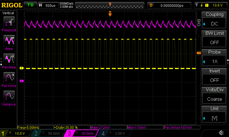
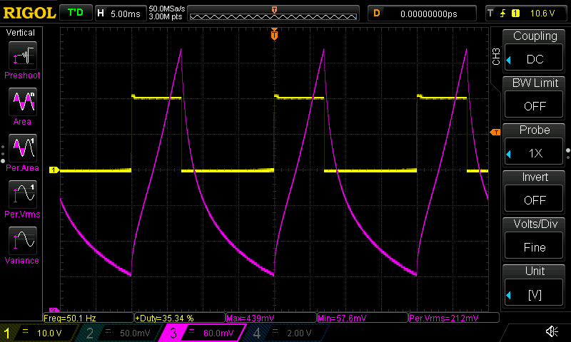
    There is another practical complication: if high-frequency PWM is applied immediately, the smoothed current does not provide a strong initial pull-in. In my testing, the solenoid struggled to pull in at 5 kHz, where it produces a relatively flat 200 mA current, insufficient for inrush current. On the other hand, at 50 Hz—same duty cycle—the current swung widely between 57 mA to 440 mA, and the solenoid was able to activate decisively.

    Running continuously at 50 Hz, however, is not the solution, because it produces an audible buzz and causes the holding force to pulsate. The practical fix is to apply a 100% duty-cycle over a short (e.g. 100 ms) activation window. More on this in the Experimental Results section below.

Pros: The circuit is simple. All it requires is a PWM control signal, a low-side N-MOSFET, and a flyback diode. The holding current is easily adjustable in software.

Cons: PWM continuously switches the solenoid voltage over potentially hundreds of feet of sprinkler wire, so EMI due to rapid voltage transitions requires serious consideration. It also becomes less convenient as the number of zones grows: either each zone needs an independently PWM-controlled switch, which rules out the shift-register architecture most multi-zone controllers use, or PWM must be introduced to the shared COM line, in which case all zones share the same duty cycle and other COM-powered accessories must tolerate the switched supply.


2. Dual-Voltage

Idea: Instead of using PWM to reduce the effective voltage, how about simply reducing the voltage itself? Apply a high voltage briefly to pull the plunger in, then switch to a stable low voltage for holding.

Reference: This is the method I adopted for the DC-powered OpenSprinkler.

Design Parameters:

  • Pull-in Voltage and Period: As in Method 1 above, a voltage between 15–24 V is generally sufficient. Applying this voltage for a short period (e.g. 100 ms), is enough to reliably pull the plunger in.
  • Holding Voltage: \( V_{\text{hold}}=I_{\text{hold}}\times R \). For a 35 Ω coil and a target holding current of 200 mA, we have \( V_{\text{hold}}=0.2\times35=7\text{V} \).

Pros: Unlike PWM, the holding voltage is steady DC, so there is no continuous high-frequency switching over long wires in the field. In addition, one power supply can serve many zones simultaneously, making the approach easy to scale to a large number of zones.

Cons: Because all zones share the same supply rail, starting a new solenoid while others are already running momentarily returns every active zone to the high pull-in current. This spike is harmless to the solenoids, but it can briefly strain an undersized power supply.

Historically, the main drawback of this method was circuit complexity. Providing two different voltage levels would require substantially more circuitry. Today, thanks to USB-C PPS, these voltages can be requested programmatically, using nothing more than a PPS-capable USB-PD sink chip like the CH224A. The implementation is surprisingly simple, and the pull-in and holding voltages can be independently adjusted with fine increments in software.


3. Synthesize AC from DC

Idea: Use an H-bridge to synthesize 24 VAC sine wave from the DC supply, and drive the solenoid with it.

Reference: The Yardian Pro Sprinkler Controller uses this approach, and appears to be the only irrigation controller on the market that does.

At first glance, this sounds counter-intuitive: didn’t we just spend all this effort ditching the AC transformer? Why convert DC back into AC now? But there are good reasons to do so.

  • Compatibility. It works not just with solenoids, but with legacy accessories like pump start relays and wireless sensors that expect a genuine 24 VAC input—some of which may not work reliably with pure DC voltage. For example, some pump start relays are large industrial contactors that have very low coil resistance and rely heavily on AC impedance to function. Under DC, they may fail to actuate or draw a massive current. Recreating an AC sine wave provides broader compatibility with the existing ecosystem.
  • Zero Net DC. Long irrigation wires often run underground and may eventually develop a nicked splice in wet soil. Sustained DC across such connections can trigger electrochemical corrosion and eat the copper. An alternating waveform leaves zero net DC and prevents this type of corrosion.
  • Modern Fault Protection. Synthesizing AC allows implementing active current limiting, short-circuit and other fault protections that are harder to achieve with a traditional AC transformer.

Design Parameters:

  • Supply Voltage. To synthesize a sine wave at 24 V RMS, the peak voltage should be \( V_{\text{peak}}=\sqrt{2}\,V_{\text{RMS}} \) \(= \sqrt{2}\times 24\approx 34\,\text{V} \). Yardian uses a 36 VDC adapter, the closest off-the-shelf DC adapter.
  • Output Frequency. This should be 50–60 Hz to match sprinkler solenoids specs.
  • Carrier Frequency. The sine wave is synthesized by rapidly switching the supply voltage at tens of kHz (carrier frequency) while modulating the duty cycle (or pulse density) according to a sine-wave envelope. A higher frequency produces lower distortion, but increases switching losses and high-frequency emissions. Conversely, a lower carrier frequency produces greater ripple and a rougher approximation of a sine wave.

Pros: This method provides the closest electrical equivalent to a traditional AC transformer. As explained above, it offers broad compatibility with existing 24 VAC accessories, leaves zero net DC in the wiring, and allows for fast modern fault protection.

Cons: The implementation is substantially more complicated than Methods 1 and 2. It requires an H-bridge, suitable gate driving, carefully designed output filter, and continuous high-frequency modulation, typically demanding a dedicated waveform generator. In addition, as the output is AC, in a multi-zone setup, zone switching needs TRIACs (instead of MOSFETs), adding cost, size, and conduction loss. Finally, a 36 VDC adapter is not common. While USB-C can provide this voltage, doing so requires an EPR-capable source of high power (e.g. 180 W), which itself is large, uncommon, and expensive.


4. Bipolar Square Wave

Idea: While experimenting with Method 3, an obvious question occurred to me: if all we really want from AC is alternating polarity, do we need to synthesize a sine wave at all? What if the H-bridge simply flips the DC polarity back and forth? The result is a bipolar square wave. It preserves the “zero net DC” property of AC, but eliminates the high-frequency carrier and much of the circuit complexity of Method 3.

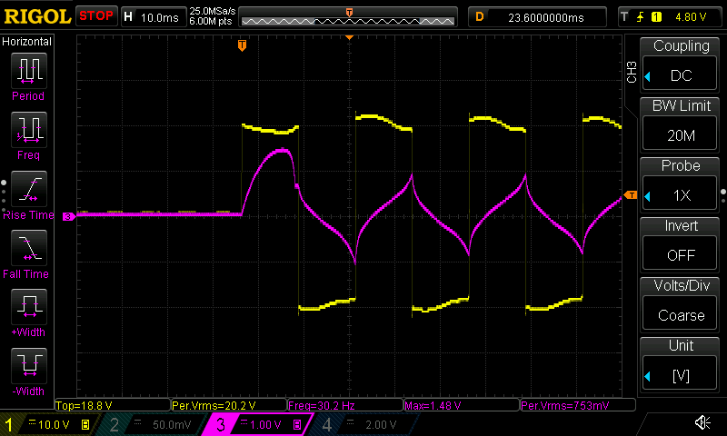
Of course, the big question is whether a sprinkler solenoid designed for sine wave would tolerate such a waveform. There is encouraging news: although the voltage is a crude square wave, the current is not. As the solenoid is strongly inductive, its current changes gradually, producing a distinctive rounded “shark-fin” waveform, as shown later in Experimental Results. To my delight, this method works remarkably well.

Design Parameters:

  • Supply Voltage. As in Methods 1 and 2 above, a fixed voltage between 15–24 V is generally sufficient. Unlike a sine wave, where the peak and RMS voltages differ by a factor of \( \sqrt{2} \), here the peak and RMS voltages are equal.
  • Output Frequency. This is a critical parameter. As the waveform is no longer sinusoidal, the ideal frequency is not necessarily 50–60 Hz. Increasing the frequency gives the inductive current less time to rise during each half-cycle and therefore reduces its RMS value. As shown in the derivation below, for typical sprinkler solenoids driven from \( \pm20V \) square wave, the optimal frequency falls in a surprisingly narrow range of roughly 40–45 Hz.

Pros: Compared to Method 3, implementation is dramatically simpler. The H-bridge only needs to reverse polarity at a low frequency; there is no high-frequency carrier or sine-wave modulation. A 20 V USB-C PD supply is sufficient, instead of the less common 36 V source. The alternating polarity also preserves AC’s “zero net DC” benefit, which reduces corrosion. Finally, with only a few dozen polarity reversals per second, switching losses and high-frequency emission are much lower than with Methods 1 and 3.

Cons: The main open question is accessory compatibility. A 40–45 Hz square wave is quite different from the 50–60 Hz sine wave that 24VAC accessories are designed for. In my testing, a heavy-duty pump-start relay (Furnas 45EG20AJ) worked reliably and its holding current at 45 Hz matches its normal holding current, which is an encouraging result. However, broader testing is still needed, especially for other pump-start relays, wireless sensors, and transformer-coupled accessories. Next, the low-frequency square wave also produces some audible hum, although subjectively it is comparable to the same solenoid running on a conventional AC transformer. Finally, because the output is AC, multi-zone switching still requires TRIACs, just as in Method 3.

Frequency Derivation: This part is math-heavy, so I kept it separate. With the help of ChatGPT, I found out that for an ideal series R-L solenoid driven by a bipolar square wave of amplitude \( V \) and frequency \( f \), the steady-state RMS current is: $$ I_{\text{RMS}} = \frac{V}{R}\sqrt{1 – 4f\frac{L}{R}\tanh\left(\frac{R}{4fL}\right)} $$

Here the seated inductance \( L \) can be estimated from the solenoid’s holding current:

$$ L = \frac{1}{2\pi f_{\text{AC}}} \sqrt{\left(\frac{V_{\text{AC}}}{I_{\text{hold}}}\right)^2 – R^2}$$

As an example, a \( R = 35\,\Omega \) solenoid drawing \( I_\text{hold}=200\,\text{mA} \) from \( V_{\text{AC}} = 24\,\text{V} \) at \( f_{\text{AC}}=60\,\text{Hz} \) corresponds to about \( L=305\,\text{mH} \) of inductance.

Now drive this solenoid with \( \pm20V \) bipolar square wave and solve the RMS-current equation for a target holding current of \( I_{\text{RMS}}=200\,\text{mA} \), we have \( f\approx 43.7 \,\text{Hz} \). 

Repeating this calculation over typical coil resistances from 25 Ω to 60 Ω gives optimal frequencies of approximately 40–45 Hz. The plot below shows how surprisingly narrow this range is.
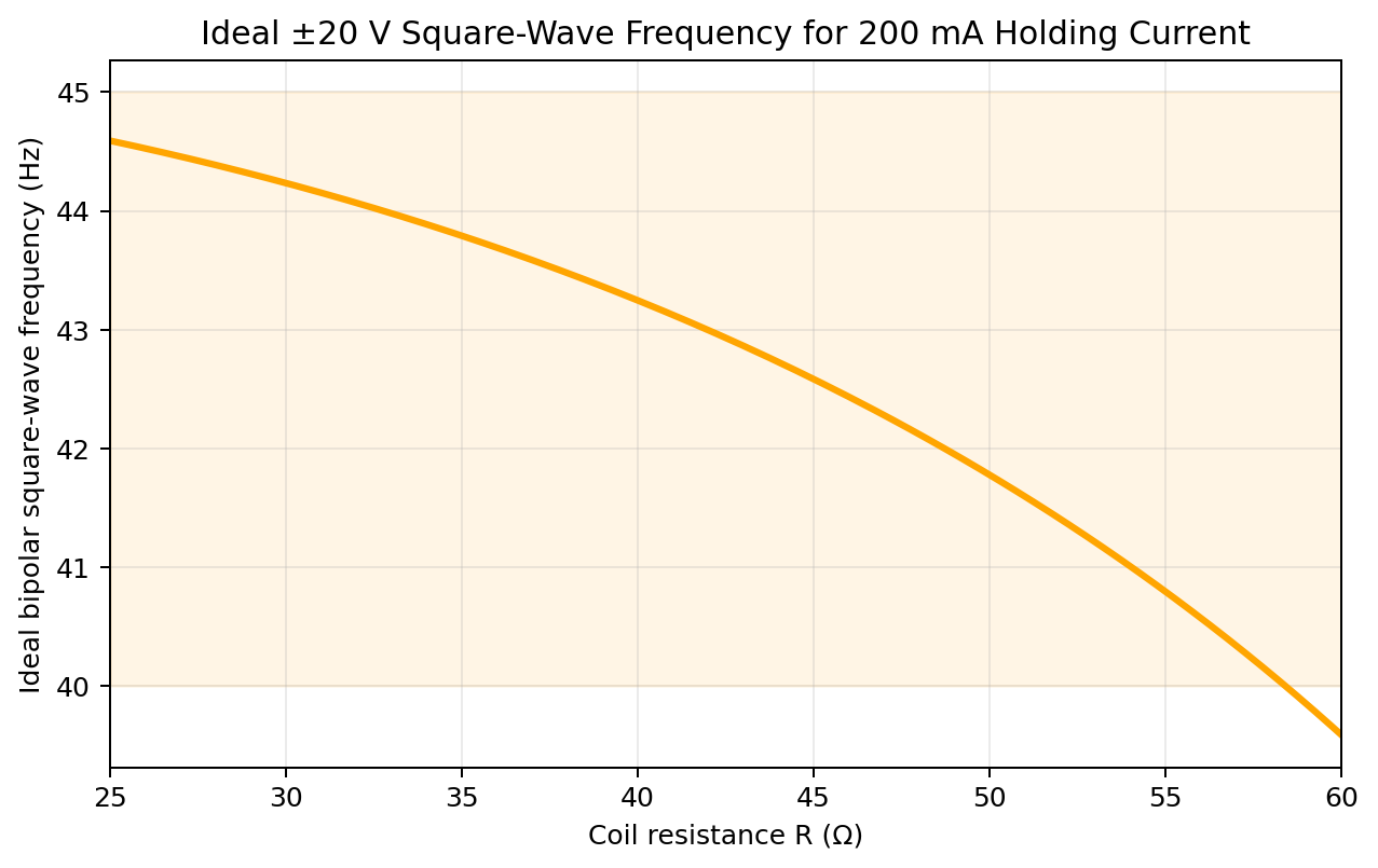
Ideal square-wave frequency to match 200 mA holding current

There is a useful intuition for why this range is so narrow. In the limit of a highly inductive coil, the square-wave voltage produces a triangle-wave current. Equating its RMS value to the current produced by a 24 VAC sine wave at 60 Hz makes the inductance cancel out entirely, leaving $$ f=\frac{2\pi\cdot 60\cdot V}{4\sqrt{3}\cdot V_{\text{AC}}} $$ For a \( V=20\,\text{V} \) supply, this evaluates to 45.3 Hz. In other words, for a strongly inductive load, a \(\pm20V\) bipolar square wave at 45.3 Hz delivers the same RMS current that the coil would draw from 24 VAC at 60 Hz. Real coils have finite resistance, which shifts the equivalent frequency somewhat lower. As a typical 24 VAC solenoid is indeed strongly inductive, this explains why different solenoids all tend to converge on the same 40–45 Hz band.


Other Methods

Two other methods are worth mentioning, although I exclude them from the main comparison because their operating parameters are largely fixed in hardware rather than adjustable in software.

Single Fixed Voltage. This is a popular DIY approach — just use a 12 VDC adapter. With a 35 Ω coil, that gives about 340 mA, a compromise that’s barely enough for inrush current and unnecessarily high for holding current. Method 2 addresses exactly this problem by using dual voltages.

Series Resistor + Bypass Capacitor. Another approach uses a series resistor to limit holding current and a capacitor in parallel with it to provide a temporary high-current path during pull-in, as demonstrated in this Hackaday project. It is simple and requires no software control, but the capacitor is bulky, the resistor dissipates heat throughout the watering cycle, the RC values are hardcoded in hardware, and the capacitor needs time to discharge before the next activation.


Implementation

To compare the four methods, I designed a single PCB containing a USB-C connector, a CH224A PD sink chip (set up in I2C mode), switching regulator, 3.3V LDO, ESP8266 microcontroller, and a discrete MOSFET H-bridge. A 1Ω resistor is placed in series with the solenoid, which lets me watch the current waveform on a scope and measure RMS current. The schematic and assembled board are shown below.
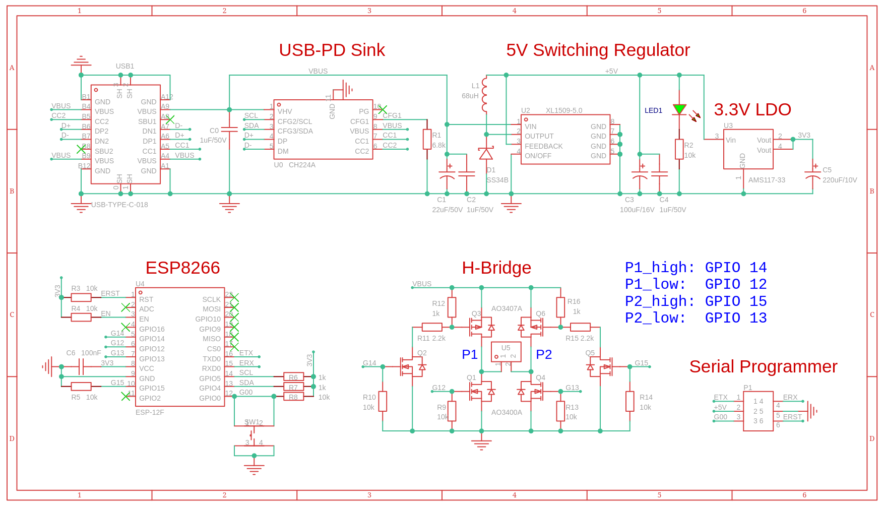
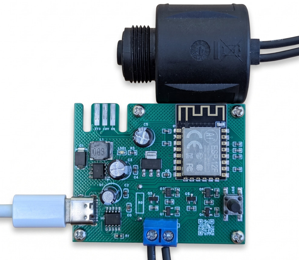
The solenoid for testing is an Orbit 24 VAC solenoid with a measured coil resistance of about 35 Ω. The power supply is a 35 W USB-PD adapter capable of 20 V/1.75 A, with PPS from 3.3–11 V.

H-Bridge. For proof of concept, I intentionally kept the H-bridge simple. Each low-side switch is an AO3400 logic-level N-MOSFET rated at 30 V (Vds); each high-side switch is an AO3407 P-MOSFET, driven by an AO3400 inverter and a 1 kΩ / 2.2 kΩ divider. All four switches are active-high and driven from four separate GPIOs, which I denote as P1_high, P1_low, P2_high, P2_low.

There is no dedicated gate-driver IC, so dead-time control is all implemented in software. This kept the prototype inexpensive. A more serious implementation should use a proper half-bridge gate driver with built-in dead-time control.

The MCU. ESP8266 is arguably not a great MCU for this experiment, particularly Method 3, for which ESP32 would be a far better choice as it provides hardware PWM peripherals. I chose ESP8266 simply because I have a drawer full of them, and it is nonetheless adequate for a proof of concept.

Configurations for the Four Methods:

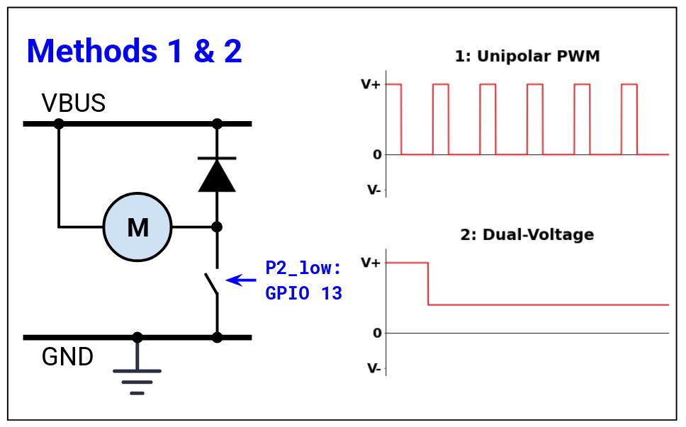
For Methods 1 and 2, only unipolar DC drive is needed. Therefore I replaced P1_high with a direct connection to VBUS, removed P1_low, and replaced P2_high with a flyback diode. P2_low is then the only active switch.

For Methods 3 and 4, the full H-bridge is populated. Method 3 uses high-frequency bridge modulation to synthesize a sine-wave, while Method 4 simply flips the supply polarity at a low frequency.

The configurations of the four methods are illustrated below.
Method 3 Implementation. This is the most software-intensive of the four methods. I had Codex implement a sine-wave synthesis algorithm using a 40 kHz, 1-bit sigma-delta pulse-density modulator. During each half-cycle, one high-side MOSFET remains on while the diagonally opposite low-side MOSFET is switched with a pulse density proportional to the magnitude of a 60 Hz sine wave; the active bridge diagonal determines the polarity. The solenoid’s inductance filters this high-frequency pulse stream into an approximately sinusoidal current. A 25μs all-off dead time is inserted whenever the bridge changes polarity to avoid shoot-through.

Download the Source Code:

Source code for all four methods is available on GitHub.


Experimental Results

1. Unipolar PWM

I started Method 1 with a PWM frequency of 5 kHz, and used an oscilloscope to measure the solenoid voltage (yellow) and current (magenta). The current was measured through the 1 Ω resistor, so 1 mV is 1 mA of coil current. The first screenshot below shows the result. Here the voltage waveform is effectively filtered by the solenoid inductance, resulting in a very smooth current waveform. But this smooth current never rises significantly above the holding level, so the solenoid struggled to pull in.

At 50 Hz PWM frequency, the result was the opposite: the much longer PWM intervals allow the current to rise substantially during each pulse, producing much stronger pull-in force (magnetic force scales with the square of current). The solenoid activated decisively. However, it also buzzes audibly.
At 1 kHz, the current ripple is clearly visible but still short of reliable pull-in. This frequency also falls within the audible range and produces a noticeable tone.
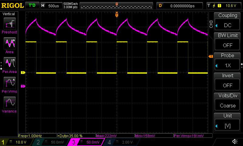
The practical solution is to separate the pull-in and holding phases: apply 100% duty cycle briefly (e.g. 100 ms) to activate the solenoid, then transition to high-frequency PWM for holding. This approach is also used in commercial solenoid drivers. For example, Vin the Wrench’s DC conversion used the DRV103 driver which has built-in pull-in delay before switching to PWM holding.


2. Dual-Voltage

The dual-voltage method is much simpler to characterize because the solenoid is driven by steady DC rather than a switching waveform. The screenshot below shows the transient behavior: initial pull-in at 20 V for 100 ms, followed by a transition to 7 V. The solenoid voltage trace is yellow, and the current is magenta.
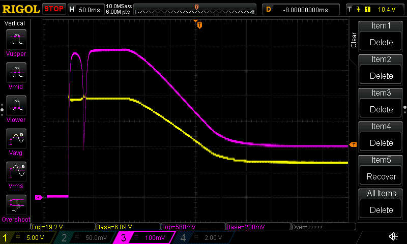
The measured peak and holding currents closely match the expected values (570 mA and 200 mA). Two observations are worth noting:

  • The current waveform reveals the mechanical action of the solenoid. After the initial current rise, a sharp dip appears as the plunger moves into position and changes in the coil inductance momentarily oppose the current. The width of this dip shows that the pull-in event completes within 50 ms.
  • The transition from 20 V to 7 V took approximately 250 ms. This delay is caused by the USB-PD adapter renegotiation process rather than the solenoid driver circuit. I confirmed this because the transition from the initial voltage ramping up to 20 V also took about 250 ms. One consequence is that the coil sees elevated current for roughly 350 ms rather than the 100 ms requested — harmless thermally, but longer than planned.

This experiment demonstrates the key advantage of the dual-voltage approach: the pull-in and holding are handled directly through voltage control, without PWM switching or high-frequency current ripple.


3. Synthesize AC from DC

A note on the supply voltage first. Producing a genuine 24 V RMS sine wave requires a 33.9 V supply. The USB-C adapter I have available tops out at 20 V, and the MOSFETs on the prototype circuit are rated for only 30 V. I therefore ran this experiment at the same 20 V used for the other methods. The synthesized waveform here should be viewed as a proof of concept rather than a full-power 24 VAC-equivalent implementation. Nonetheless, it illustrates the essential behavior of the method.

The first capture below shows that although the voltage is generated by high-frequency switching, the current waveform is much smoother and resembles a sine wave. The coil’s inductance does the filtering, exactly as intended. Measured RMS current is 107 mA at 59.9 Hz.

The second capture zooms in on the voltage waveform. The pulse density varies across each half-cycle — dense near the peak, sparse near the zero crossing — which is what the sigma-delta modulator produces. Note also the phase lag: the current crosses zero well after the voltage flips polarity, as expected for an inductive load.
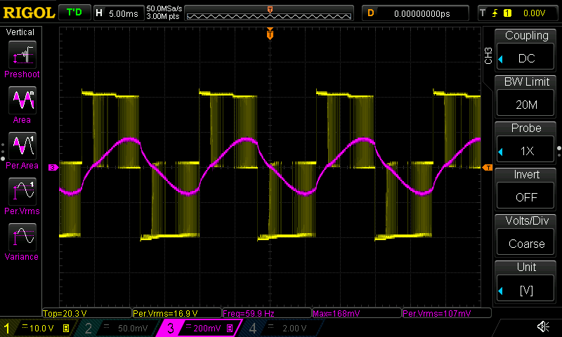
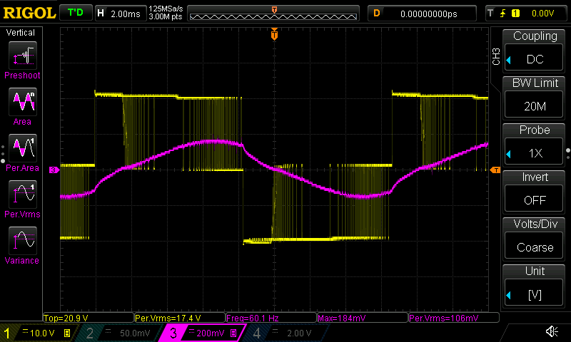
The third capture was taken with the plunger held out, and the current is substantially larger (341 mA). This demonstrates the inrush-versus-holding behavior: with the plunger out, inductance is lower, impedance is lower, and the coil draws more current. In addition, as resistance dominates, the phase lag is much less pronounced. Once the plunger seats, the inductance rises and the current naturally falls. This is the key feature of traditional AC drive: the transition from high inrush current to lower holding current happens automatically, without any pull-in timing phase in software.
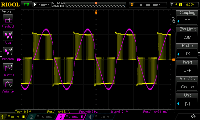
Although the experiment used a 20 V supply (for reasons explained above), the results can be roughly extrapolated to a 33.9 V supply, which is \(33.9/20 \approx 1.695\) times higher. Assuming the solenoid behaves approximately linearly, the measured currents would scale up to about 181 mA holding and 578 mA inrush, close to the solenoid’s rated values.


4. Bipolar Square Wave

This is perhaps the most interesting method. The drive itself is substantially simpler than Method 3, yet the result still closely resembles what the solenoid sees under true AC. Because the square wave’s frequency directly affects RMS current, I collected results at three frequencies: 40, 45, and 50 Hz.

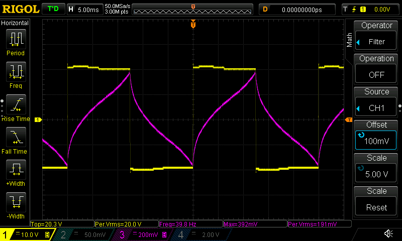
I started at 40 Hz (\(\pm20V\)). The first capture below shows the holding state with the plunger seated. The RMS current is 191 mA. While the voltage is a crude square wave, the current takes on a much smoother “shark-fin” shape, showing the expected exponential rise and fall during each half-cycle.

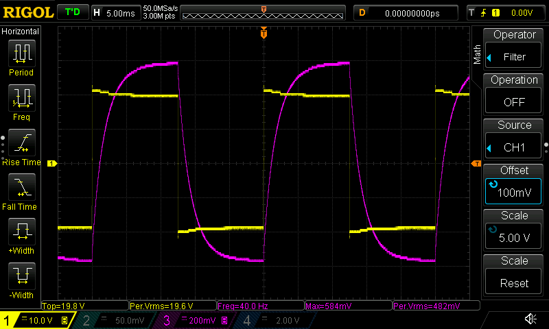
To check the inrush behavior, I physically held the plunger out, and the RMS current increased dramatically to 482 mA, as shown in the second capture. This closely resembles the natural inrush-to-hold behavior of the solenoid under conventional AC drive.
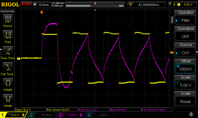
The pull-in capture below shows the transition from inrush to holding as the plunger moves into position. The current peaks at about 568 mA, and the pull-in event completes in roughly 20–30 ms.
So far the sprinkler solenoid behaves well under bipolar square-wave. But what about other 24 VAC accessories, such as pump-start relays? They may have very different coil resistance and inductance.

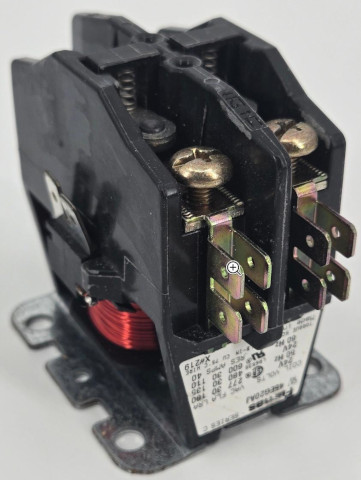
To find out, I hooked up a Furnas 45EG20AJ pump-start relay. This is a heavy-duty contactor with a coil resistance of only about 9 Ω and a rated holding current of 300–330 mA. At 40 Hz bipolar drive, it pulled in decisively and held reliably, but drew about 399 mA RMS, above its normal AC holding current. During pull-in, the current rose to roughly 1.48 A peak, then dropped sharply as the contactor closes and the coil inductance rises.
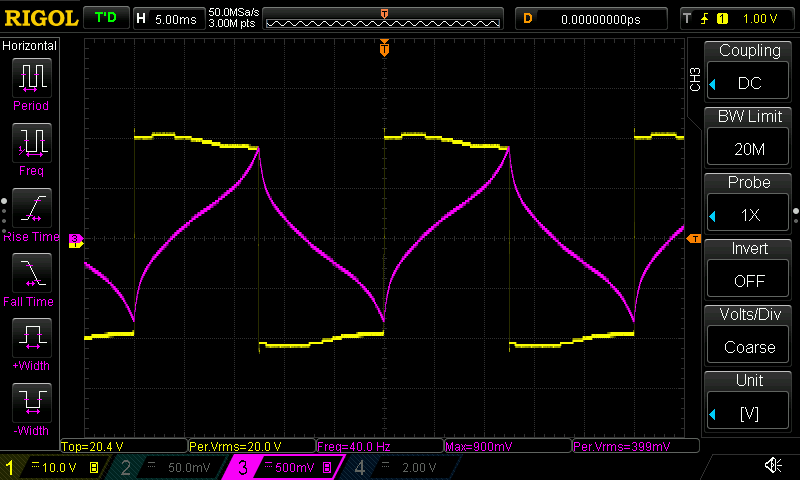
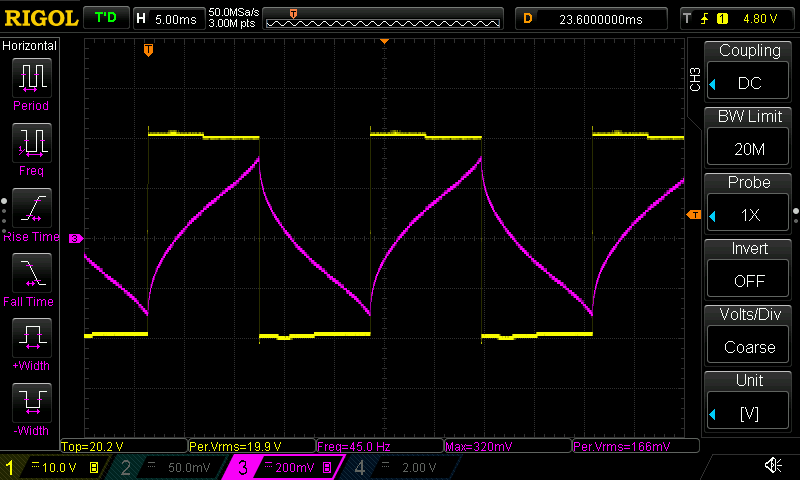
Next, I increased the square wave frequency to 45 Hz. The sprinkler solenoid’s holding current drops to 166 mA, and the Furnas relay to 329 mA. This is particularly interesting because it closely matches the theoretical prediction discussed earlier: for a strongly inductive load, 45.3 Hz is the frequency at which a \(\pm20V\) bipolar square wave delivers the same RMS current as a 24 VAC, 60 Hz sine wave.

For reference, I measured the Orbit solenoid and the Furnas relay driven from three conventional 60 Hz transformers. Interpolating the measurements to 24 VAC (since no single transformer produced precisely 24 VAC) gives approximately 165 mA RMS for the solenoid and 330 mA RMS for the relay. In comparison, the 45 Hz square wave produces 166 mA and 329 mA respectively—both remarkable matches. Two devices differing by a factor of four in coil resistance, both reproduced almost exactly.
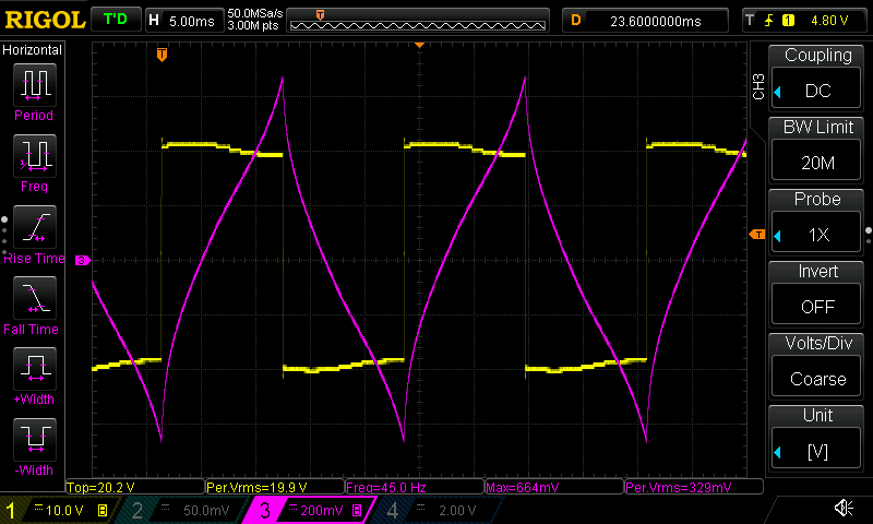
Finally, I increased the square wave frequency further to 50 Hz. The sprinkler solenoid current drops to about 148 mA RMS, while the Furnas relay to about 287 mA RMS. Both are noticeably below their normal operating currents, although pull-in and holding remained reliable for both.
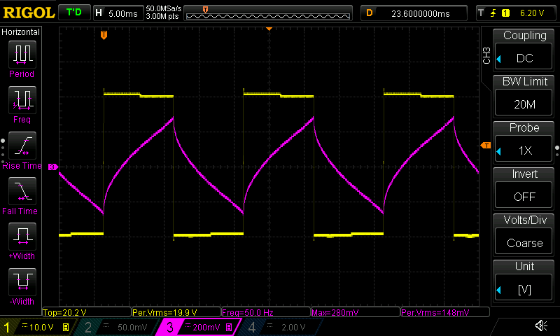
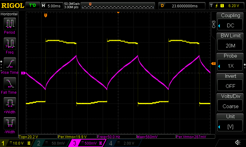
Discussion. The measurements are summarized below:

FrequencySolenoidRelayObservation
40 Hz191 mA399 mABoth somewhat over-driven
45 Hz166 mA329 mABoth within 2% of their 24 VAC values
50 Hz148 mA287 mABoth somewhat under-driven, but still reliable
24 VAC reference165 mA330 mAmeasured 24VAC / 60 Hz results

Overall, the measurements agree remarkably well with the theory. Increasing frequency reduces RMS current because the current has less time to build during each half-cycle. Moreover, 45 Hz is a sweet spot: for both the sprinkler solenoid and the much heavier Furnas contactor, the measured RMS current closely matches what they draw from a traditional 24 VAC sine wave transformer.

Compatibility with arbitrary 24VAC accessories is still not guaranteed, but the successful Furnas test is encouraging because it represents exactly the sort of heavy pump-start contactor that would be difficult to drive using the DC-only methods.


Conclusion

There is no single best method here: each trades simplicity, flexibility, and compatibility differently. Choose:

  • Unipolar PWM if you want the quickest prototype and the least hardware complexity. A single MOSFET and flyback diode are enough, and holding current is easy to adjust in software. The tradeoff is continuous high-frequency switching.
  • Dual-Voltage if you want similarly simple hardware but prefer steady DC output. With USB-C PPS, both voltages can be easily adjusted in software.
  • Sine-Wave AC Synthesis if you want genuine 24 VAC output, zero net DC on the field wiring, and maximum compatibility with existing AC accessories. But it comes with the highest hardware and software complexity.
  • Bipolar Square Wave if you want most of what Method 3 offers without most of what it costs. It preserves zero net DC, automatic inrush-to-hold, likely good compatibility with existing 24 VAC accessories, and only requires the H-bridge to flip polarity at a few dozen Hz. The trade-offs are that there is audible buzz, and broader accessory compatibility needs further testing.

USB-C is what makes all of this practical. Even when a method uses a fixed drive voltage, USB-C PD lets the controller select among several supply voltages without changing adapters; with PPS, it can be adjusted in fine increments. Combined with universal 100–240 V input, regulation, built-in protection, compact size, and near-universal availability, USB-C turns out to be a surprisingly capable replacement for the old 24 VAC transformer—one you may finally be ready to ditch.


Tags: , , , , , , ,

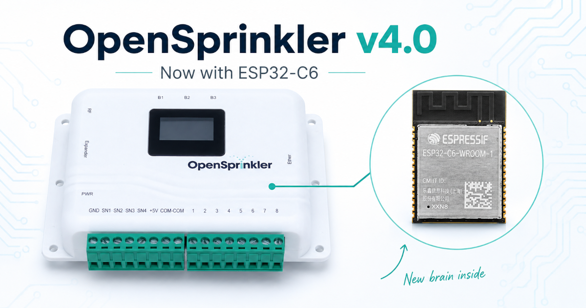
Exciting news! We’re getting ready to launch the next generation of OpenSprinkler: AC-Powered OpenSprinkler v4.0, the first built on ESP32. From the outside it looks just like v3.4 — same enclosure and same ports — but inside is an entirely new brain, with a faster processor, more memory and flash space, WiFi 6, analog inputs, native USB, and radio hardware that opens the door to Matter, Thread, and Zigbee.

We’re accepting pre-orders now, with shipments expected in late September 2026.


TL;DR — What’s New in OpenSprinkler v4.0?

  • ESP32-C6 replaces ESP8266 – A faster and more capable MCU with substantially more RAM and flash, WiFi 6, offering better compatibility with modern routers and mesh networks.
  • Improved security – Hardware-accelerated encryption and modern security features provide a stronger foundation for secure network connections.
  • Built-in analog sensor inputs – Thanks to plentiful ADC-capable pins, all four built-in sensor ports (SN1–SN4) can be individually configured as either digital or analog input (0–3.3V).
  • Built-in USB-C port – Native USB CDC means no separate USB-serial programmer needed for firmware recovery or debugging.
  • Matter / Thread / Zigbee-ready – ESP32-C6 is equipped with a 802.15.4 radio. Firmware support for these features is planned for future releases.
  • Same accessory compatibility – Fully compatible with existing Zone Expander (v3), the newly debuted Sensor Expander, and the W5500 wired Ethernet module.

Goodbye ESP8266, Hello ESP32

The ESP8266 has served OpenSprinkler remarkably well since v3.0 was released ten years ago. It is inexpensive, reliable, has built-in Wi-Fi, and remains surprisingly capable for such a small microcontroller.

But technology moves on. Espressif has officially listed ESP8266 as Not Recommended for New Designs, and many new IoT products have long since migrated to the ESP32 family.

Moving to ESP32 gives OpenSprinkler considerably more headroom. The ESP32-C6 has a 160 MHz RISC-V processor, 512 KB of SRAM, many more peripherals, ADC channels, native USB, and modern wireless capabilities. As OpenSprinkler firmware has grown over the years, we’ve added more networking features, sensor support, integrations, and increasingly sophisticated web. ESP32-C6 gives us substantially more room to continue developing these features without constantly worrying about resource constraints.


Fun Fact About Version 3.4

When I announced OpenSprinkler v3.4 last year, there was an embarrassing little truth: v3.4 was never supposed to exist! The original plan was to go directly from v3.3 to v4.0, with v4.0 being the first ESP32-based OpenSprinkler.

The problem was deciding which ESP32.

You see, when ESP8266 arrived, it had no variants. The decision was a no-brainer because there was nothing else to choose. ESP32, on the other hand, has close to a dozen variants, so many that they’re organized into whole series: S, C, H, P. Usually, having choices is a good thing. Having too many choices, however, causes confusion and exhaustion — evaluating all of them and working out which was best for OpenSprinkler took me a lot of reading and several rounds of prototyping.

I eventually settled on the C6, because it hits a sweet spot: ample GPIOs, plenty of memory and processing power, WiFi 6, hardware-accelerated encryption, and the 802.15.4 radio. It doesn’t have the raw horsepower of the S series, and it lacks the 5 GHz WiFi of the C5 — but neither matters much for a sprinkler controller, so those were easy trade-offs to accept.

The result of all that deliberation was roughly a year of delay, and v3.4 became the transition release that filled the gap. Classic paralysis by too many choices. But I’ve finally caught up, and OpenSprinkler v4.0 is just around the corner!


Questions You May Have

Q: When will v4.0 be available?
A: We’re accepting pre-orders now, with shipments expected in late September 2026.

Q: What about the OpenSprinkler DC and Latch models?
A: DC v4.0 is in development and expected to be ready by November 2026. There’s no immediate plan for a v4.0 Latch due to its relatively small demand. We will continue evaluating demand and revisit it in the future.

Q: Will v3.4 or v3.3 still be available?
A: v3.4 is a transition version and will no longer be offered once it sells out.
v3.3 will continue to be available as a replacement board (without enclosure) for repairs and DIY projects.

Q: Will v4.0 use different firmware?
A: OpenSprinkler will continue using a unified firmware codebase, so the source is the same. However, because v4.0 has a different microcontroller, the compiled binary is different. To avoid confusion, automatic firmware download and flashing will be provided as a software feature.

Q: Will you keep releasing firmware updates for v3?
A: Yes. The ESP8266 is older but still very capable, with plenty of RAM and flash headroom, and firmware development will continue for all v3 versions (v3.0–v3.4). Advanced features that depend on v4 hardware — built-in analog sensor inputs, Matter/Thread/Zigbee — will be v4-only.

Q: Can I reuse my existing Expanders and the W5500 wired Ethernet module?
A: Yes. v4.0 is fully compatible with Zone Expander v3, the recently released Sensor Expander, and it uses the same W5500 wired Ethernet module as v3.4/v3.3.

Q: Does v4.0 support 5 GHz Wi-Fi?
A: No — the ESP32-C6 is 2.4GHz only, though it does support WiFi 6 (802.11ax) and WPA3 on that band. This is a good fit for an IoT device like OpenSprinkler, where 2.4 GHz generally provides better range and wall penetration.

Q: Can I power v4.0 using the onboard USB-C port?
A: The USB-C port is used for firmware recovery (in the case of a corrupted firmware) or debugging. While it can provide power to the logic board, you still need a 24VAC transformer to operate solenoid valves.

Q: Given it has built-in analog sensor inputs, do I still need the Sensor Expander?
A: It depends on how many sensors you need. OpenSprinkler v4.0 has four built-in sensor ports, and each can be configured as either a digital or analog input. This means existing digital sensors, such as rain or flow sensors, will reduce the number of ports available for analog input. The Sensor Expander provides 16 additional analog input channels, independent of the four built-in sensor ports. So if you need more analog inputs, or want to keep the built-in ports available for digital sensors, the Sensor Expander is still the way to go.

Q: Do I need to upgrade to v4.0?
A: If your existing OpenSprinkler is working well, there is no need to upgrade just for normal sprinkler operation. v4.0 mainly provides a newer processor with more resources, analog sensor inputs, native USB, and support for future features that the v3 hardware cannot provide.

Q: I just bought an OpenSprinkler AC v3.4. Can I exchange it for v4.0?
A: Yes, as long as your purchase was made within 30 days, which qualifies under our no-questions-asked return and refund policy (see our terms and conditions).


Tags: , , , , , , ,

Some projects take a weekend. Some take a summer. And some take… a little over five years. Today I’m thrilled to make two announcements at once: OpenSprinkler Firmware 2.2.1(5) is officially available, and the Sensor Expander — after a month of pre-orders — is officially shipping.

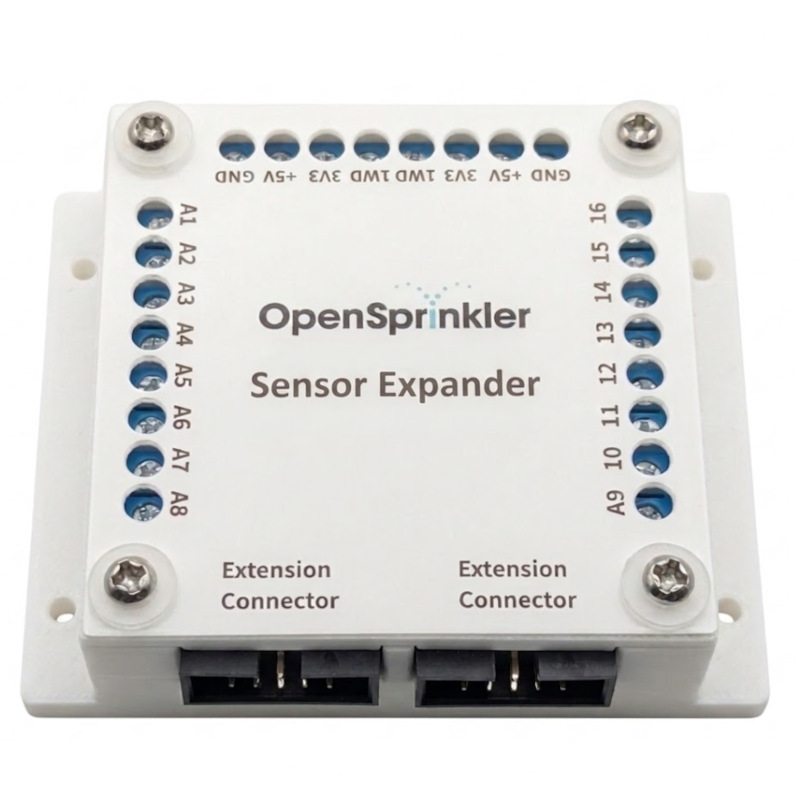
As detailed in our previous New Product Alert post, the Sensor Expander is an add-on for OpenSprinkler v3 that provides 16 channels of analog sensor input. You can plug in a variety of external sensors, such as soil-moisture, temperature, light, water-level — you name it. This allows OpenSprinkler to read, display, and log these sensors, and use them to automatically adjust programmed water times based on real-world conditions. This opens the door to more advanced irrigation applications in which watering decisions are guided by precise environmental measurements rather than simple on-or-off sensor signals.


The Backstory

What makes this release especially meaningful to me is the long journey it took to get here.

The idea for an analog sensor board based on ADS1115 goes back more than five years. You see, one long-standing limitation of OpenSprinkler has been its inability to read analog sensors. While its built-in digital sensor ports can detect binary signals (e.g. HIGH or LOW, open or closed), many environmental sensors produce a continuously varying voltage—those analog signals are essential for applications that need to measure how much moisture, light, temperature, or water is present, rather than simply whether a threshold has been crossed.

In late 2020, an idea occurred to me: OpenSprinkler’s expander port uses I²C, and many analog-to-digital converter (ADC) chips also communicate over I²C. One of the most popular choices in the maker community is the ADS1115. An expander built around that chip could give OpenSprinkler analog-input capability while still allowing Zone Expanders to share the same port.

In February 2021, I built an early prototype and demonstrated that the concept was feasible. That was in the early days of the pandemic, and I had to deal with the sudden onset of several personal issues, so unfortunately the progress on the project stalled.

Then something wonderful happened: our German distributor, Stefan Schmaltz, took my prototype and continued developing the idea. He designed his own version, implemented firmware support for it, and has sold it for the past several years as the Analog Sensor Board, or ASB. Stefan’s design repurposes the existing Zone Expander enclosure. That enclosure works nicely, but it has room for only 16 terminal ports. Including the required +5V, 3.3V, and ground terminals, the board is limited to 8 ADC input channels. Kudos to Stefan for keeping the project alive, turning the original concept into a real product, and demonstrating that there is genuine demand for analog sensor support.


From Prototype to Sensor Expander

Meanwhile, I continued sketching ideas, albeit slowly, for a more refined version. Instead of repurposing the existing Zone Expander enclosure, I envisioned a new board with its own dedicated 3D printed enclosure, and enough space for 16 ADC channels—the maximum supported by the available I²C address configurations of the ADS1115.

At the same time, I had been thinking about another recurring customer request: support for a 2-wire irrigation system in which multiple zones share the same pair of wires and are controlled through encoded signals. Such a system can greatly reduce the amount of copper wiring required for installations with many zones. With that future application in mind, I added a 1-Wire master chip to the board. It is intended to support future experimentation with 2-wire-style encoder and decoder systems, while also making it possible to interface with standard 1-Wire sensors such as the popular DS18B20 temperature sensor.

After several rounds of revisions, the hardware finally came together last year. Along the way it also went through several name changes. At first, I called it the Analog and 1-Wire Extension Board. I also considered the abbreviation OWA, for “1-Wire and Analog.” Neither name was particularly attractive or easy to understand.

Eventually—with a little help from generative AI—the obvious name emerged: Sensor Expander, a natural counterpart to the existing Zone Expander.


The Software Challenge

Finalizing the hardware was only half the story. Supporting an entirely new class of configurable, loggable, and watering-adjusting sensors required substantial changes to both the firmware and the user interface. It turned out to be a significant usability-design challenge: users needed a way to configure different sensor types, understand their readings, view historical logs, and define how each sensor should affect watering.

The software work began during the summer of last year, kick-started by my student, Andrew Friedman. Our original plan was to integrate Stefan’s OpenSprinkler ASB firmware and interface directly into the official OpenSprinkler repositories. After further consideration, we decided instead to draw on the concepts and lessons from his implementation while rewriting the firmware and user interface from scratch, to fit more naturally into the official OpenSprinkler framework.

As the summer ended, progress stalled once again while we turned our attention to several more urgent priorities: launching OpenSprinkler v3.4, in both AC and DC versions, releasing OpenGarage 2.3+, and navigating continuing supply-chain difficulties.

Then, earlier this year, we got our momentum going again—helped along in no small part by the recent leaps in generative AI and agentic coding tools, which turned many slow, repetitive firmware, interface, testing, and documentation tasks into something we could complete much more efficiently. And finish we did! During the past month, all of the final pieces came together: the Sensor Expander circuit, its dedicated 3D-printed enclosure and acrylic front cover, Firmware 2.2.1(5), the updated app/user interface, and a completely refreshed set of manuals.

From the first idea to the finished product, the journey took more than five years. It is both a genuine relief and a real thrill to finally see it cross the finish line.


What Else is New in Firmware 2.2.1(5)?

While support for the Sensor Expander is its primary addition, Firmware 2.2.1(5) also includes several other important features, performance improvements, and bug fixes.

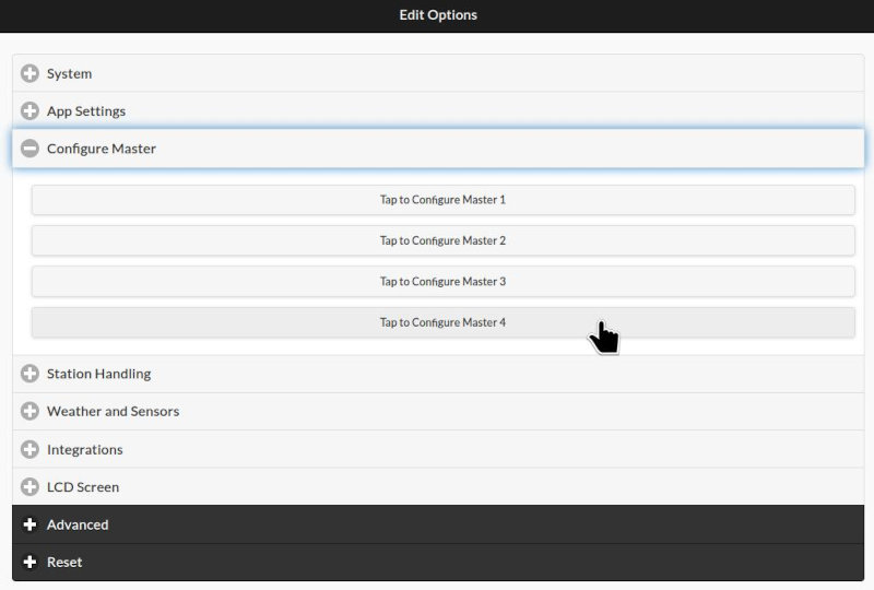
  • Support for Up to Four Master Zones, with independent on/off timing and per-zone control over Master selection. One of OpenSprinkler’s distinguishing features has always been that Master zones are defined in software. Most sprinkler controllers provide a single dedicated Master Valve (MV) terminal. OpenSprinkler instead allows any zone to be designated as a Master. The benefit of that design is especially clear with this update: you are not restricted to one fixed Master terminal, and different zones can activate different Master valves or pumps as needed.
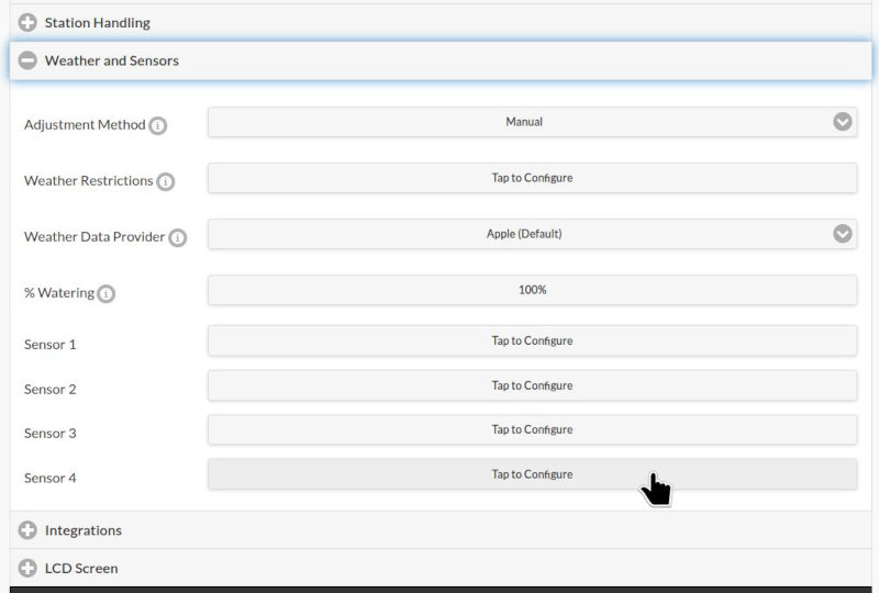
  • Two Additional Built-In Sensor Ports. OpenSprinkler v3.4 added the SN3 and SN4 ports, bringing the total number of built-in sensor ports to four. Firmware 2.2.1(5) enables these two additional ports, each of which can be configured independently as a rain sensor, soil-moisture sensor, or program switch.
  • Longer Watering Duration. While programmed water durations are still limited to 18 hours, after scaling by weather and sensor adjustments, the resulting runtime is allowed to exceed this limit, up to the firmware’s 7-day bound.
  • Updated Documentation: The documentation has been substantially refreshed and expanded. New and updated resources include the firmware User Manual, API doc, and dedicated user manuals for the Sensor Expander and Zone Expander respectively.
  • Performance, Reliability, and Bug Fixes. This firmware includes numerous performance and reliability improvements (e.g. more efficient memory allocation, reduced fragmentation, improved OTF library and streaming server output) as well as bug fixes (e.g. out-of-bound memory access involving parallel groups, repeated Run-Once program attribution, a potential station runtime overflow when adjustment exceeds 100%).

Firmware Update: Because this firmware is a build-number update, upgrading from any 2.2.1 (e.g. 2.2.1(4)) to 2.2.1(5) will preserve your existing settings, programs, and logs. No factory reset is needed. Regardless, we always recommend exporting a copy of your current configurations before updating, just in case a factory reset becomes necessary.

End of Support for OpenSprinkler v2.3: One important change is that Firmware 2.2.1(5) no longer supports OpenSprinkler v2.3 (the legacy AVR-based hardware model that was discontinued 10 years ago). Going forward, official firmware releases will continue to support OpenSprinkler v3 (v3.0-v3.4) as well as OSPI/Linux. For OpenSprinkler v2.3 users, Firmware 2.2.1(4) is the final supported firmware.


Where to Get Everything?

Finally, a big thank-you to Stefan Schmaltz and Andrew Friedman, whose work helped pioneer and advance this project.

Comments and feedback are always welcome.


Tags: , , , , , ,

A long-requested feature for OpenSprinkler is the ability to read analog sensors, including temperature, soil moisture, water level, light, and more. While OpenSprinkler’s built-in sensor ports can read binary (i.e., HIGH or LOW) signals—primarily from dry-contact switches like rain and flow sensors—it has lacked the ability to read analog sensors that produce continuous voltage signals. Analog sensors are critical for advanced irrigation applications, where users rely on precise environmental data to fine-tune their watering times.

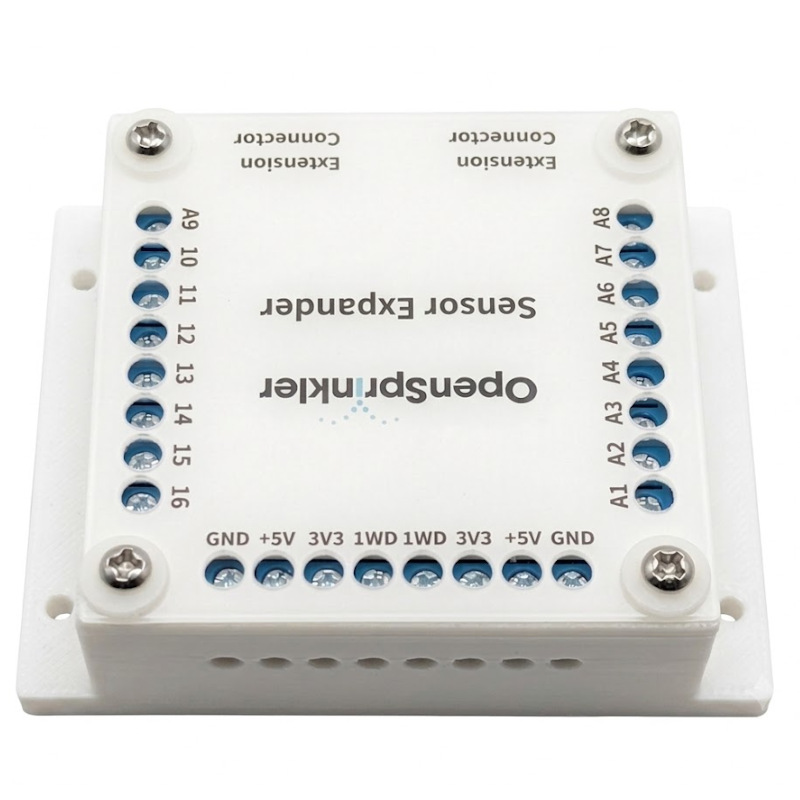
Introducing the OpenSprinkler Sensor Expander—our upcoming product that provides 16 channels of analog sensor inputs, allowing your OpenSprinkler to interface with a wide variety of external sensors and automatically adjust your programmed water times based on real-world conditions. Below are two sneak peek photos of this new expander.


Main Features:

  • 16 Analog Sensor Inputs: Powered by four ADS1115 Analog-to-Digital Converters (ADCs), providing a total of 16 independent high-precision analog sensor inputs.
  • Dual Voltage Options: Selectable 5V and 3.3V to support a wide range of sensors.
  • Easy Expansion: Plugs directly into OpenSprinkler’s Zone Expander connector using the same 2×5 ribbon cable interface. It can be used standalone with the main controller or inserted at any point in an existing Zone Expander chain.
  • Hardware 1-Wire Master: Includes an on-board 1-Wire Master controller to enable future support for 1-Wire sensors, such as the DS18B20 temperature sensor (firmware support coming soon).

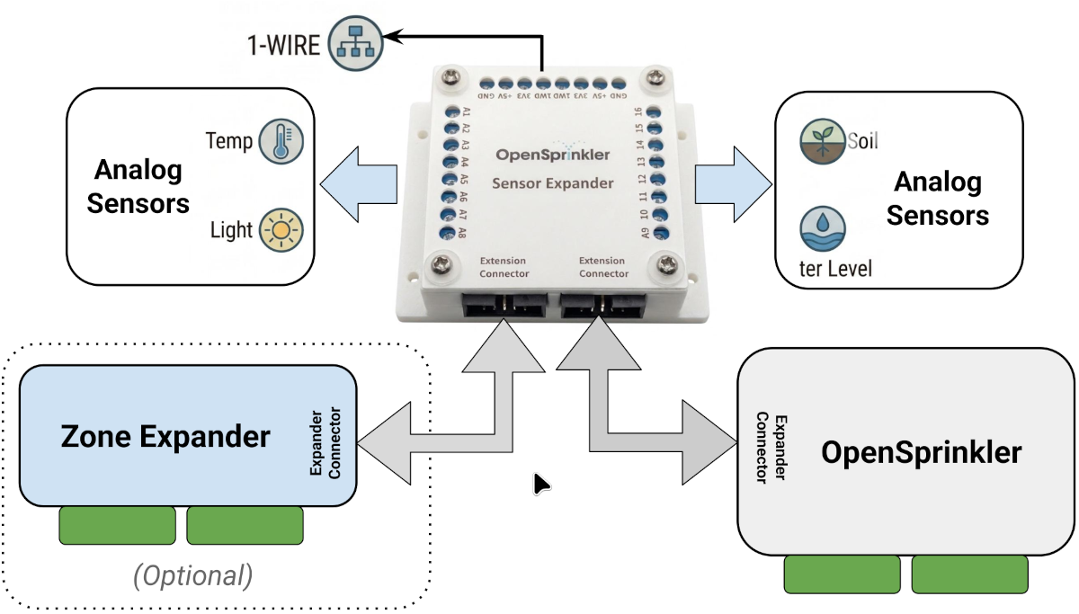
Below is an illustration of the Sensor Expander and how it connects to the OpenSprinkler main controller and (optionally) your Zone Expanders.


Firmware Support

We are actively working on finalizing OpenSprinkler firmware 2.2.1(5), which will be the first release to support the Sensor Expander. Below are several screenshots showing the new firmware user interface in action. We are currently accepting pre-orders, with a targeted shipping date of late-July 2026.


Edit Sensors Page:

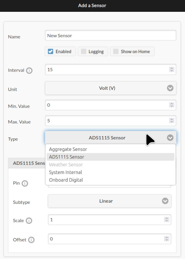
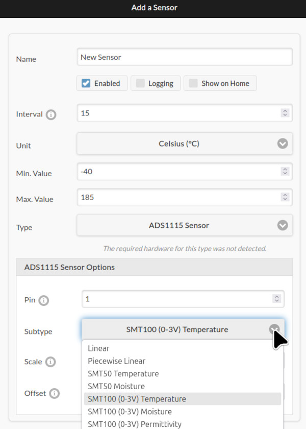
The Sensor configuration interface lets you create a new sensor or edit an existing sensor by providing a custom name, sampling interval (e.g., every 15 minutes), physical unit, min/max clamping values, and sensor type. Currently supported sensor types include:

  • ADS1115: For sensors connected to the expander’s analog inputs. Includes three sub-types:
    • Generic Linear: Define custom linear parameters (scaling and offset) that map raw ADC voltage to sensor value.
    • Baked-in Types: Pre-configured for known sensors (e.g. SMT50 and VH400), with scaling and offset parameters taken directly from the sensor datasheets.
    • Piecewise Linear: The most flexible type, supporting non-linear mapping with up to 8 sample points.
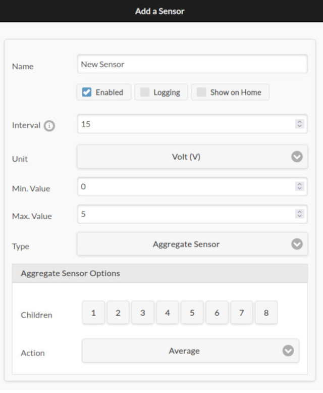
  • Aggregate Sensors: Combine up to 8 “child” sensors and aggregate their data using operations like Average, Min, Max, Median. This is useful for example, when you need to average or denoise readings from multiple soil moisture sensors. Aggregate sensors can themselves be children of other aggregate sensors, allowing flexible hierarchies.
  • On-Board Digital Sensors: Allows you to programmatically link the controller’s internal digital sensors (e.g., rain, soil) to the new Sensor interface. Normally, on-board sensors affect watering on a per-zone basis (via each zone’s ‘Ignore Sensor’ flag). By routing them through the Sensor interface, you can use them in program-level adjustments.
  • System Internal Sensors: Monitor metrics like available Heap size and Flash size. Combined with logging, this lets you track the microcontroller’s resource usageover time.

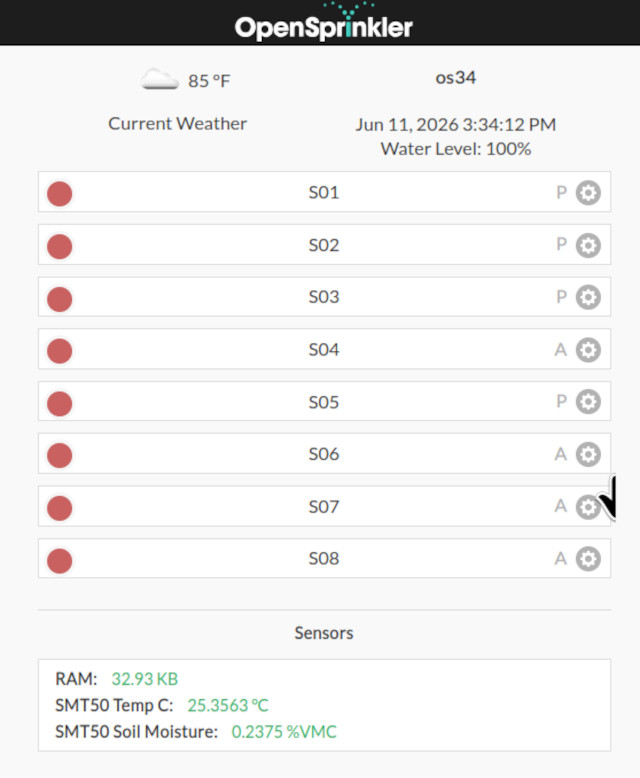
Note: Firmware 2.2.1(5) supports up to 64 sensors total, each with configurable parameters such as logging and the option to display on the home page, as shown below.


Sensor Logs Page:

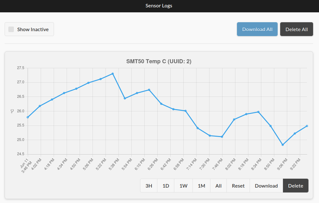
The Sensor Logs page displays logged data from all active sensors that have ‘Logging’ flag enabled. You can select different time windows to zoom into specific periods, download the logs as .csv files for external analysis, or delete the logs of individual sensor. A “Show Inactive” checkbox lets you view logs from disabled or previously deleted sensors.


Sensor Adjustments in Edit Programs Page:

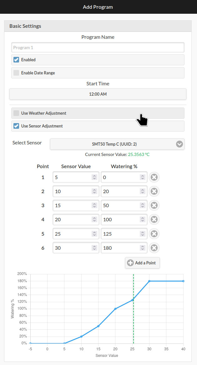
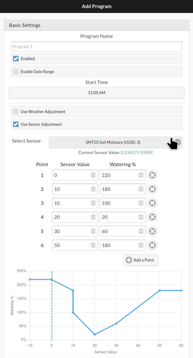
The Edit Programs page now includes a new ‘Sensor Adjustment‘ section. It lets you define how the program’s water times should be modified based on the value of a selected sensor. For example, reducing watering when soil moisture is high, or increasing it when temperature is warm. You can use any sensor as input, including an Aggregate Sensor that combines readings from multiple sources.

In this interface, you can select a sensor and configure a custom Adjustment Curve using up to 8 sample points, defining how sensor readings translate into watering percentages. The adjustment curve is visualized in real-time, with the current sensor value shown as a green dotted line for reference.

Sensor Adjustment works alongside the existing Weather Adjustment feature. The program’s final water time is multiplied by both the sensor-based percentage and the weather-based ‘watering level’.


Other Firmware Features:

Beyond Sensor Expander support, firmware 2.2.1(5) brings several additional enhancements, including support for up to 4 Master Zones (previously 2), and up to 4 on-board digital sensors on hardware v3.4 (previously 2).


FAQ:

Q: What are some example use cases for the Sensor Expander?
A: The Sensor Expander is particularly useful when you want to modify watering times based on real-world sensor readings — for example, reducing watering when soil moisture is high, adjusting for temperature and evaporation, accounting for ambient light levels, or stopping irrigation when a water tank runs low.

Q: Which OpenSprinkler hardware is compatible with the Sensor Expander?
A: The OpenSprinkler v3 family (v3.0 through 3.4) is compatible. The Sensor Expander uses the same 2×5 ribbon cable connector as the v3 Zone Expanders.

Note that OpenSprinkler v2.3 and OpenSprinkler Pi (OSPi) are NOT compatible with the Sensor Expander. However, recent versions of OSPi (v1.5 and v2.0) feature two on-board ADS1115 chips, providing 8 channels of analog inputs out of the box when updated to firmware 2.2.1(5).

Q: When will the Sensor Expander be ready to ship?
A: We are taking pre-orders now! Shipping is expected to begin in late-July 2026.

Q: What types of sensors are supported?
A: Most analog sensors that operate on 3.3V or 5V logic are supported. Popular examples include the Truebner SMT50, SMT100, Vegetronix VH400, and many resistive and capacitive moisture sensors. The Generic Linear and Piecewise Linear sensor types provide flexibility to support virtually any analog sensor by configuring custom mapping parameters.

Q: What’s the size and weight of the Sensor Expander?
A: The Sensor Expander measures 80mm × 65mm × 30mm (3.15in × 2.56in × 1.18in) and weighs 75g (2.65oz).

Q: If I use the Sensor Expander, can I still use Zone Expanders?
A: Absolutely! The Sensor Expander works alongside Zone Expanders. They both utilize the same I2C communication bus, meaning multiple devices can be connected on the same chain. You can have one Sensor Expander plus multiple (up to 4) Zone Expanders, in any order along the chain.

Q: Can I daisy-chain two Sensor Expanders to get 32 analog inputs?
A: Unfortunately, no. Each main controller can only support one Sensor Expander. The ADS1115 chip allows only 4 unique I²C addresses, and our Sensor Expander already uses all four, so there is no capacity for any additional. If you require more than 16 analog inputs, you will need to add a second OpenSprinkler main controller with its own Sensor Expander.

Q: Can I connect digital sensors (e.g., rain sensor, flow sensor) to the Sensor Expander?
A: While switch-type sensors (like rain and flow) can technically be connected to the expander, we highly recommend using the main controller’s dedicated on-board digital sensor inputs instead. The Sensor Expander inputs have heavy low-pass filtering and slow sampling rates, optimized for analog measurements rather than fast digital signals.

Flow sensors should NOT be connected to the Sensor Expander. The combination of slow sampling and heavy filtering will cause missed pulses, making accurate flow measurement impossible. Connect flow sensors to the main controller’s on-board sensor inputs.

Q: Can I use custom sensors not in the pre-defined list?
A: Yes! The Generic Linear sensor type lets you configure custom linear mapping (scaling and offset) for any analog sensor. For sensors with non-linear response curves, the Piecewise Linear sensor type supports up to 8 sample points for arbitrary mapping. Your sensor’s datasheet generally provides the formula. Alternatively, an empirical approach is to measure your sensor’s output voltages at known reference values, and use the collected voltage-value pairs to define the Piecewise Linear curve.

Q: What’s the 1-Wire Master for?
A: The Sensor Expander includes an on-board 1-Wire master controller, capable of processing the 1-Wire communication protocol. But firmware support for 1-Wire sensors (such as the DS18B20 temperature sensor) is not yet implemented. We plan to add this in a future firmware update.


Ready to add intelligent sensor-based irrigation to your OpenSprinkler? Pre-order the Sensor Expander now and be among the first to receive it in late-July 2026!

Tags: , , ,

A common question we receive from users is: “How do I use OpenSprinkler to switch a water pump, a heater, a fan, or similar mains-powered devices?” Here are the top 5 ways to bridge the gap between OpenSprinkler and your high-voltage equipment, ranging from “Zero Wiring” to “Zero Software Configuration“.


1. WiFi Smart Plugs

  • Best For: Ease of use, zero wiring, and total safety.
  • Approx. Cost: ~$20

This is rapidly becoming the most popular method because it requires zero physical wiring between the controller and the pump. You can have your OpenSprinkler in the garage and control a pump in a greenhouse 50 feet away.

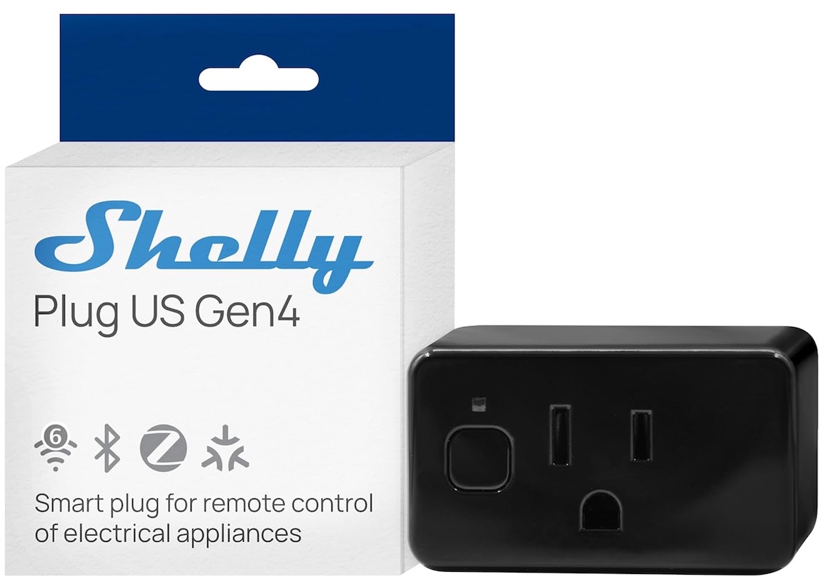
How does it work: WiFi power sockets like the Shelly Plug US support a well-documented HTTP API, which allows you to send commands over WiFi to switch the socket on or off. Crucially, they allow for local IP-based control without relying on a cloud server—a perfect solution for privacy-focused users.

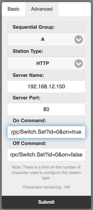
OpenSprinkler features a station type called “HTTP Station“, which sends user-defined HTTP commands when a zone opens or closes. By leveraging the smart plug’s API, zone actions transfer directly to the power plug.

Shelly US Plug Gen 4
HTTP Station Config

How to set it up:

  1. Configure your WiFi plug to connect to your router and obtain its IP address.
  2. In OpenSprinkler, edit a zone and set its Station Type to HTTP.
  3. Enter the plug’s IP address and Port in the Server Name and Port fields.
  4. Configure the HTTP commands. Using the Shelly US plug as an example:
    • On command: rpc/Switch.Set?id=0&on=true
    • Off command: rpc/Switch.Set?id=0&on=false
  5. Test the zone to verify the plug responds. (Note: If you use a different brand, check its API documentation for the correct command path).

Pros:

  • Galvanic Isolation: Complete air-gap isolation. No risk of messing with high-voltage wires.
  • Expandability: Easy to expand to multiple plugs / pumps. You aren’t limited by the physical ports on your OpenSprinkler unit.
  • Power Monitoring: Many plugs include power consumption monitoring.

Cons:

  • Not all WiFi plugs support HTTP API or local IP-based control.
  • Relies on your WiFi router (if WiFi is down, the pump won’t turn on).
  • Requires initial WiFi configuration on the plug.

2. Wireless but No WiFi: RFToy and RF Sockets

  • Best For: Long-range control where WiFi is weak.
  • Approx. Cost: ~$40 (RFToy + Sockets)

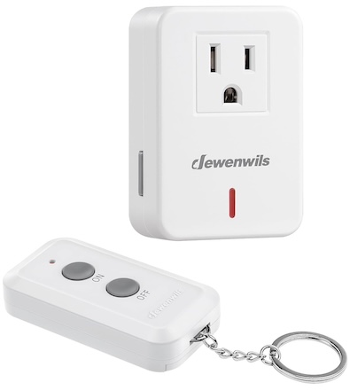
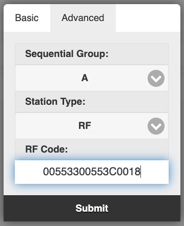
RF Power Sockets work on the 433MHz or 315MHz bands (unlike the 2.4GHz used by WiFi) and typically come with a dedicated remote. With an RFToy, you can decode the remote’s signal and replicate it using OpenSprinkler. OpenSprinkler’s ‘RF Station’ feature is designed exactly for this. You paste the code that RFToy intercepted from the remote, allowing the zone to toggle the socket.

RF power socket with remote
OpenSprinkler RF Station Config

Pros:

  • Range: RF signals often penetrate walls and floors far better than WiFi.
  • Isolation: Complete air-gap isolation. No wiring required.
  • Cost: RF sockets are cheaper per unit than WiFi plugs, making expansion more affordable.

Cons:

  • Requires purchasing an extra device (RFToy)
  • Usually one-way communication (no feedback signal to confirm the plug actually turned on).

3. The Safe Wired Way: IoT Relay

  • Best For: Users who want a reliable wired-only connection without messing with mains voltage.
  • Approx. Cost: ~$40

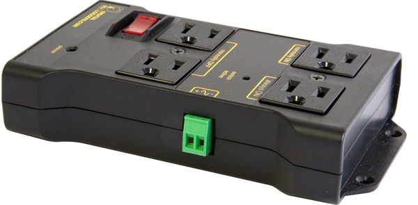
If you prefer the reliability of a wired connection but are uncomfortable stripping 110V wires, the IoT Relay is great. It looks like a power strip but features a green low-voltage terminal block on the side.

How to set it up:

  1. Run two wires from OpenSprinkler (COM and a Station Port) to the green connector on the IoT Relay. It works with both AC-powered and DC-powered OpenSprinkler units.
  2. Plug your pump into the “Normally OFF” outlet.
  3. When the station activates, the outlet turns on.

Pros:

  • Zero Software Configuration: No WiFi configuration to manage.
  • Plug-and-Play: UL-listed and fully enclosed. Safe to use.
  • Reliable: It’s a hardwired connection, so it works even if your WiFi goes down.

Cons:

  • Current limit: Limited to ~12 Amps, which may not meet your pump’s specs.
  • Availability may be limited as there is only one manufacturer.
  • Expanding Cost is High if you need to switch multiple pumps.

4. The DIY Way: 24VAC Relay / Solid State Relay (SSR)

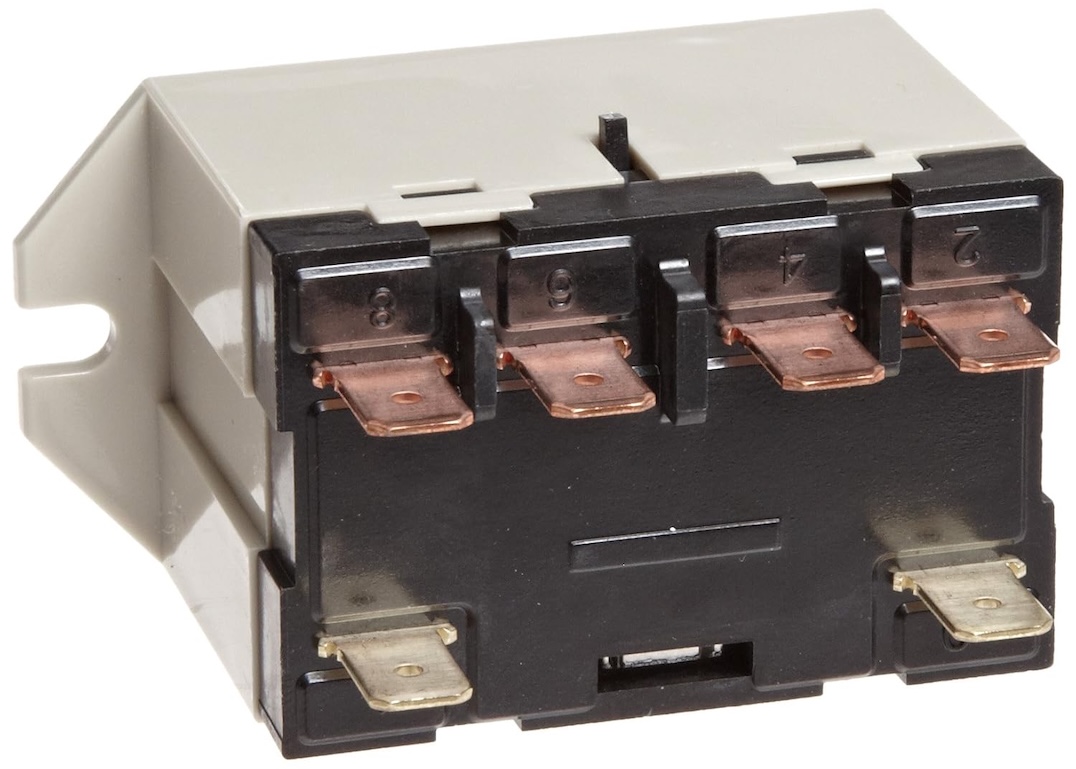
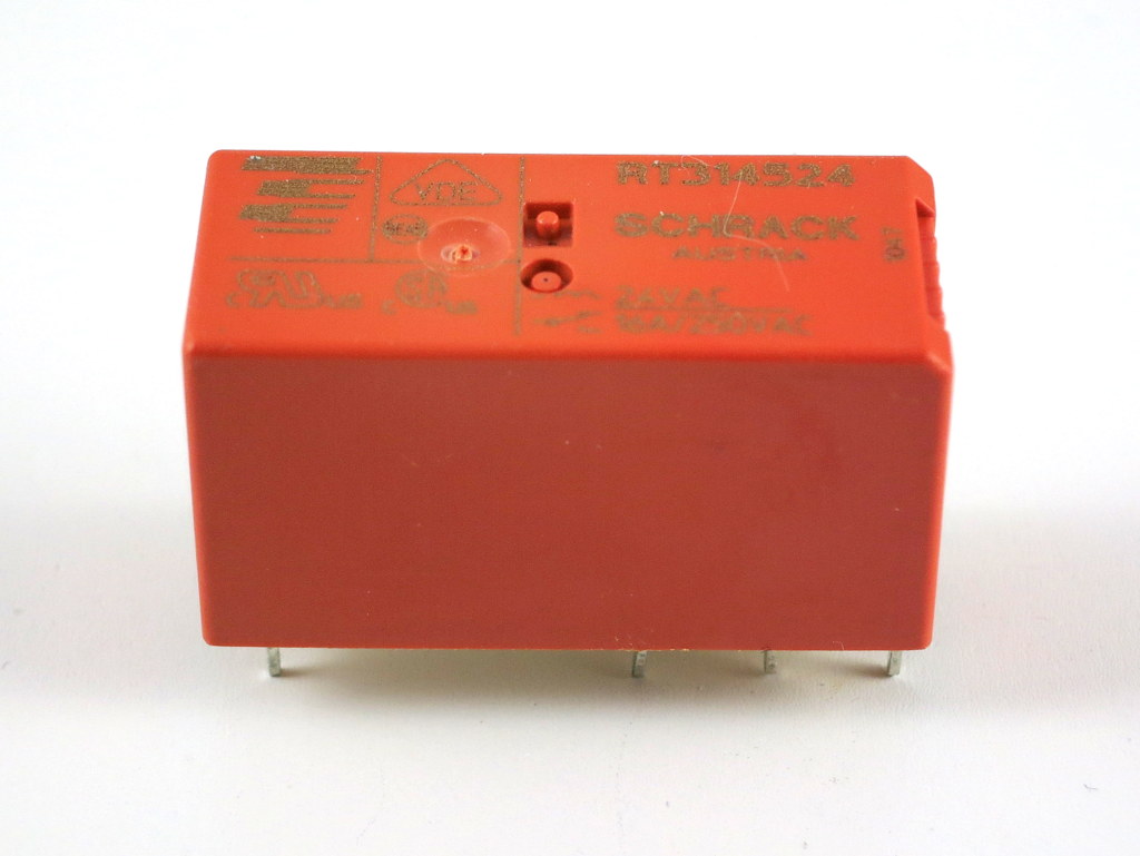
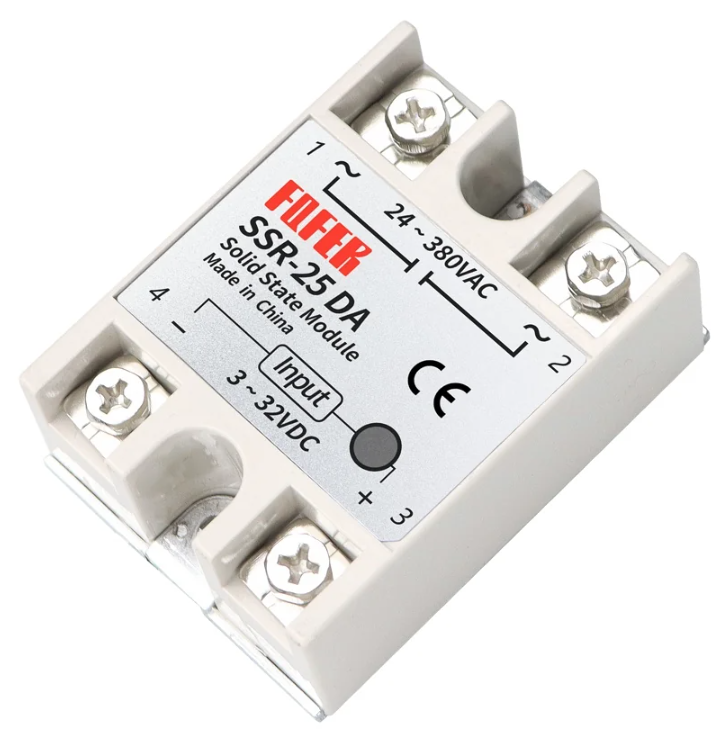
This is the classic “old school” approach. You buy a standard relay with a 24VAC Coil (for AC-powered OpenSprinkler only; or, if using a DC-powered OpenSprinkler, get a DC Solid State Relay). You wire the coil to the OpenSprinkler just like a sprinkler valve, and wire your pump through the relay’s switch contacts.

Pros:

  • Lowest Cost: The cheapest option by far.
  • Reliable: Hardwired connection works even if WiFi fails.

Cons:

  • Safety Hazard: Requires proper enclosure and handling of exposed mains voltage.
  • Wiring Required: You need to handle both low and high voltage wiring.

5. The Heavy Duty Option: Pump Start Relay

  • Best For: Large (1HP+), high power (>1500W), or 3-phase pumps
  • Approx. Cost: ~$50–$80

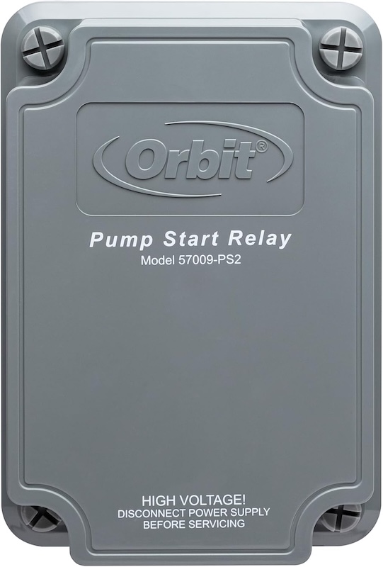
If you are running a massive well pump or a booster pump for a large lawn, small relays will weld shut due to the “inductive kickback” of the motor. You need a dedicated Pump Start Relay (from brands like Orbit, Hunter, or Rain Bird). These are essentially industrial-grade versions of Option 4, housed in a NEMA-rated outdoor box.

Pros:

  • Robust: Built to handle the massive in-rush current of large pumps.
  • Code Compliant: Safe for permanent outdoor installation.

Cons:

  • Most expensive option.
  • Requires professional hardwiring.
  • Expansion cost is very high.

Summary & Comparison

MethodBest ForWiring EffortSoftware ConfigIsolationCostExpansion Cost (unit)
Shelly / WiFi PlugEase of useNone (Wireless)Medium (WiFi+HTTP setup)Excellent (Air Gap)~$20Medium (~$20)
RFToy+SocketRangeNone (Wireless)Low (RF setup)Excellent (Air Gap)~$40Low (<$10)
IoT RelayWired SafetyLowNoneGood (Internal)~$40High (~$40)
24VAC Relay / SSRLow Cost DIYHigh (Mains Voltage)NoneGood (Coil)~$5Low (~$5)
Pump Start RelayHeavy DutyMediumNoneGood (Coil)> $40High (>$40)

Tags: , , ,

Older Posts »